Model diagrams and equations, straight from the code
The figure and the math in your report should never disagree with the model you ran
By Matthew Fidler in nlmixr2 rxode2
September 29, 2026
Many pharmacometric reports have the same two items near the top of the methods section: a compartment diagram of the final model and the equations that define it. They are also two of the easiest things to get wrong.
The diagram is usually drawn by hand in PowerPoint or Visio early in the analysis. The equations are typed into Word or LaTeX from the control stream. Then the model changes – a transit compartment is added, the effect goes from stimulation to inhibition, a covariate moves – and the code is updated but the figure and the math are not. A reviewer who reads the equations in the report and the code in the appendix will find two different models.
The fix is to generate both from the model itself. nlmixr2plot
5.2.0 adds automatic compartment diagrams, and nlmixr2extra can
already turn a model into LaTeX equations. Since both read the same
model object you fit, they cannot drift from it.
Compartment diagrams with modelDiagram()
Take the classic two-compartment model with first-order absorption:
two.cmt <- function() {
  ini({
    tka <- log(1.5)
    tcl <- log(3)
    tv <- log(20)
    tq <- log(2)
    tvp <- log(40)
    eta.ka ~ 0.1
    eta.cl ~ 0.1
    add.sd <- 0.2
  })
  model({
    ka <- exp(tka + eta.ka)
    cl <- exp(tcl + eta.cl)
    v <- exp(tv)
    q <- exp(tq)
    vp <- exp(tvp)
    d/dt(depot) <- -ka * depot
    d/dt(central) <- ka * depot - cl / v * central - q / v * central +
      q / vp * periph
    d/dt(periph) <- q / v * central - q / vp * periph
    cp <- central / v
    cp ~ add(add.sd)
  })
}
One call draws it:
modelDiagram(two.cmt, engine = "ggplot2")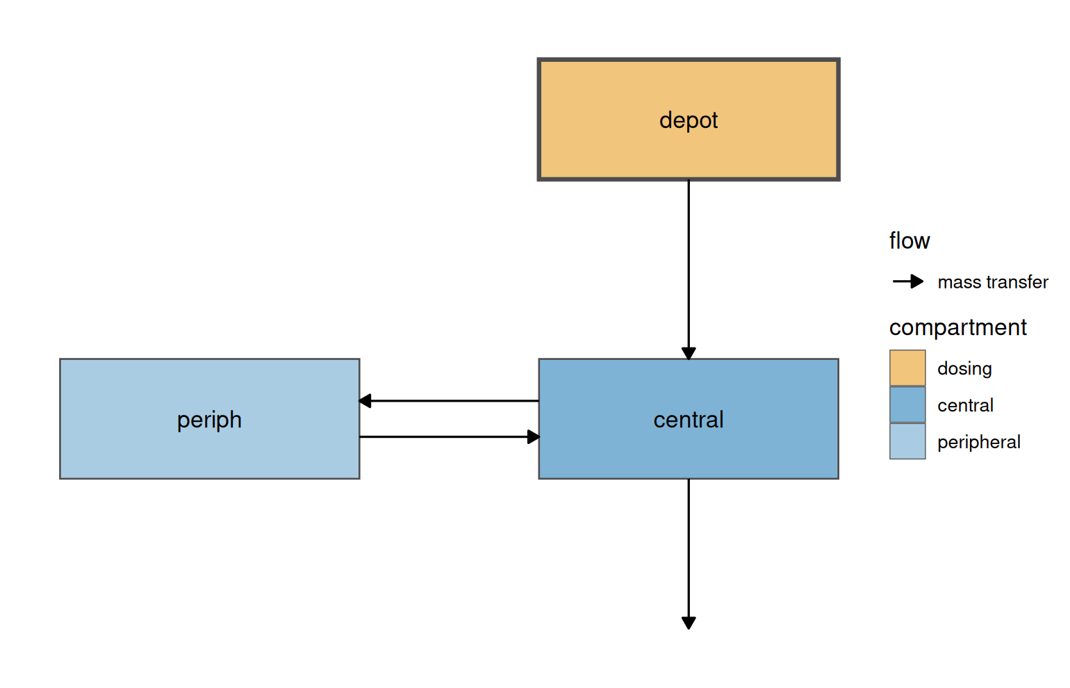
There is no layout information in the model. modelDiagram() reads
the d/dt() equations, works out which terms move mass between
compartments, and places the compartments the way a pharmacometrician
would draw them by hand: the dosing compartment (heavy border) on top,
peripheral compartments to the left, elimination leaving the central
compartment downward.
For a methods section you often want the rate terms (the model expressions that drive each flow) on the arrows too:
modelDiagram(two.cmt, engine = "ggplot2", labels = TRUE)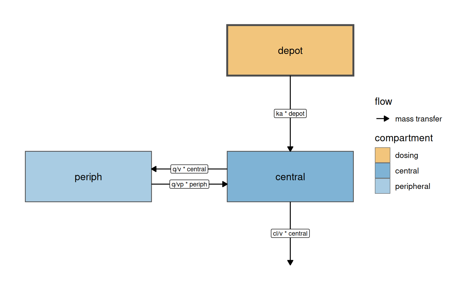
plot() of an rxode2 model object draws the same diagram, so
plot(rxode2(two.cmt), engine = "ggplot2") works as well. (A fit
keeps its goodness-of-fit plot(); use modelDiagram(fit) for its
diagram.)
Behind the picture, modelGraph() returns the parsed compartments and
flows as data frames, which is handy for checking how the equations
were read, or for drawing them some other way.
In the development version of nlmixr2plot, these labels are colored white, but this can still be immediately useful even if you don’t install the development version.
Three engines, three kinds of report
The engine argument decides what you get back, and each one fits a
different reporting workflow:
"ggplot2"returns an ordinaryggplotobject. Theme it to match the rest of your figures, save it withggsave()at the resolution your publisher asks for, or put it side by side with a goodness-of-fit plot usingpatchwork."DiagrammeR"(the default when ‘DiagrammeR’ is installed) gives an interactive Graphviz widget, handy in HTML reports and Quarto dashboards."dot"returns the Graphviz DOT source as text. When the automatic layout is 95% of the way there, this is the escape hatch: edit the DOT and render it with any Graphviz tool, rather than starting a drawing from scratch.
cat(modelDiagram(two.cmt, engine = "dot"))## digraph model {
## graph [layout = neato, splines = true, outputorder = edgesfirst, forcelabels = true];
## node [shape = box, style = "rounded,filled", fontname = Helvetica];
## edge [fontname = Helvetica, fontsize = 10];
## "depot" [pos = "0,1.1!", fillcolor = "#F2C57C", penwidth = 2];
## "central" [pos = "0,0!", fillcolor = "#7FB3D5"];
## "periph" [pos = "-1.67,0!", fillcolor = "#A9CCE3"];
## "depot" -> "central";
## "central" -> "periph" [dir = both];
## ".elimination4" [shape = point, style = invis, width = 0.01, pos = "0,-0.77!"];
## "central" -> ".elimination4";
## }Not just PK
The part that saves the most time is the pharmacodynamic side, where hand-drawn diagrams are fiddliest. Terms that influence a compartment without moving mass into it – effect compartments, stimulation and inhibition of turnover – are drawn as dashed or dotted arrows, and the direction of the effect is read from the equation itself. Here is an indirect response model where the drug inhibits production of the response:
pk.turnover <- function() {
  ini({
    tktr <- log(1)
    tka <- log(1)
    tcl <- log(0.1)
    tv <- log(10)
    poplogit <- 2
    tec50 <- log(0.5)
    tkout <- log(0.05)
    te0 <- log(100)
    prop.err <- 0.1
    pdadd.err <- 10
  })
  model({
    ktr <- exp(tktr)
    ka <- exp(tka)
    cl <- exp(tcl)
    v <- exp(tv)
    emax <- expit(poplogit)
    ec50 <- exp(tec50)
    kout <- exp(tkout)
    e0 <- exp(te0)
    DCP <- center / v
    PD <- 1 - emax * DCP / (ec50 + DCP)
    effect(0) <- e0
    kin <- e0 * kout
    d/dt(depot) <- -ktr * depot
    d/dt(gut) <- ktr * depot - ka * gut
    d/dt(center) <- ka * gut - cl / v * center
    d/dt(effect) <- kin * PD - kout * effect
    cp <- center / v
    cp ~ prop(prop.err)
    effect ~ add(pdadd.err)
  })
}
modelDiagram(pk.turnover, engine = "ggplot2")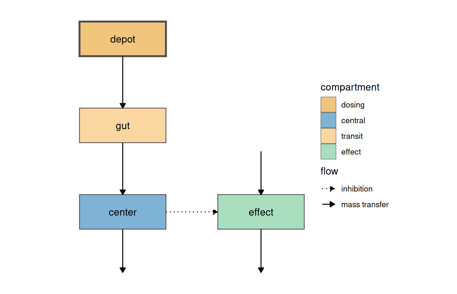
Nobody told it that effect is a turnover response, that gut is a
transit compartment, or that the drug is inhibitory. It followed PD
back through DCP to center, saw that PD falls as the
concentration rises, and drew an inhibition. If you later change the
model to a stimulatory effect, the diagram changes with it.
Target-mediated drug disposition works the same way; binding and unbinding are recognized as mass moving from both partners into the complex and back out again:
tmdd <- rxode2::rxode2({
  d/dt(central) <- -kel * central - kon * central * target + koff * complex
  d/dt(target) <- ksyn - kdeg * target - kon * central * target +
    koff * complex
  d/dt(complex) <- kon * central * target - koff * complex - kint * complex
})
modelDiagram(tmdd, dosing = "central", engine = "ggplot2")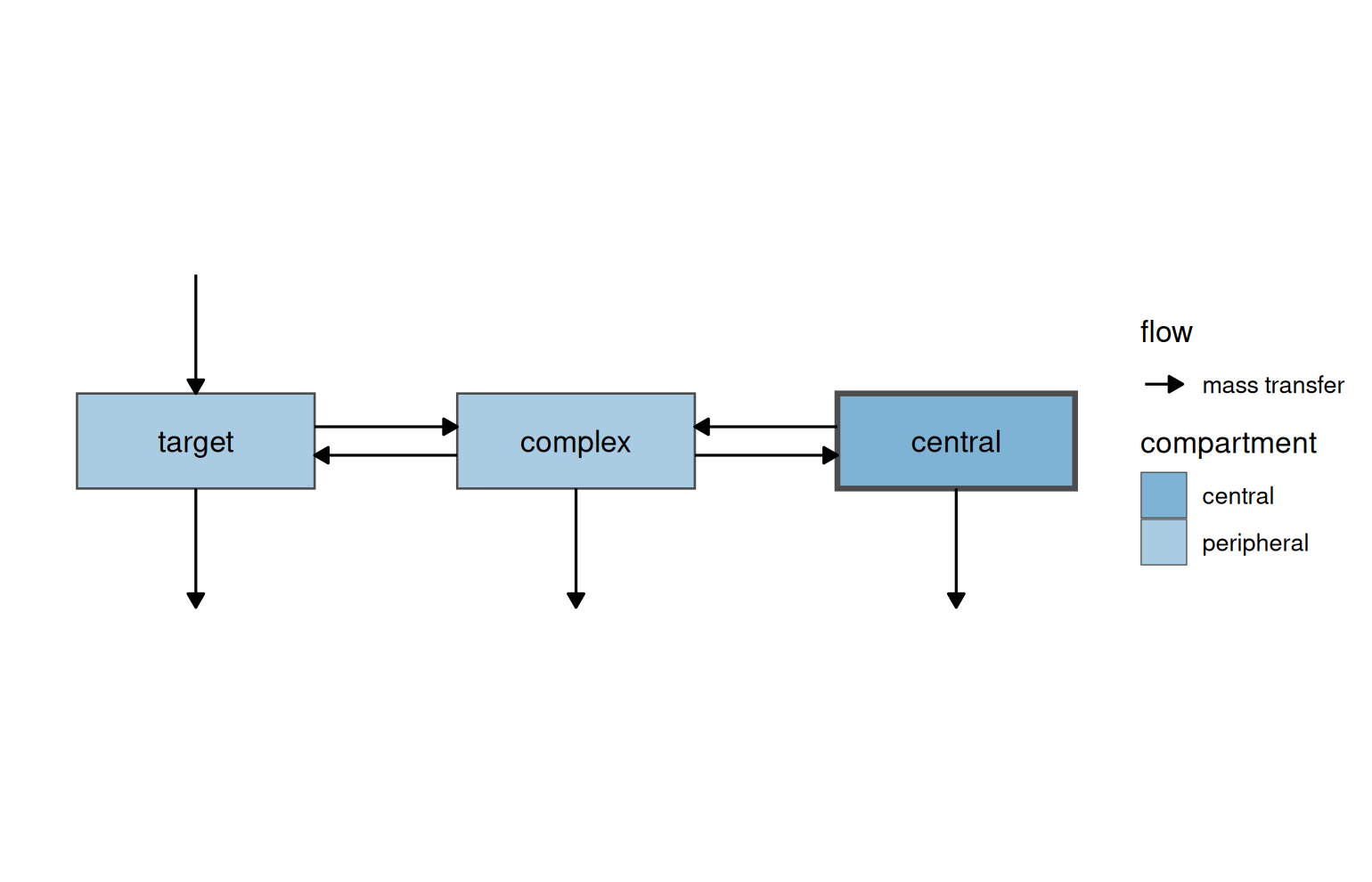
Before release, the diagrams were checked against all 3043 models in
nlmixr2lib, including large
QSP and PBPK models. The Automatic model diagrams
vignette
covers the rest: how each term is classified, lag()/f()/rate()/dur()
annotations, delay(), linCmt() models, and the current limitations.
Model equations with knit_print()
nlmixr2extra has a knit_print() method for rxode2 model objects
created from a model function (rxode2(fun)) and for nlmixr2 fits. In practice that means that when a model or fit is
the last value of a chunk in R Markdown or Quarto, the chunk prints the
model as aligned LaTeX equations instead of as R code:
rxode2::rxode2(two.cmt)\[\begin{align*} {ka} & = \exp\left({tka}+{eta.ka}\right) \\ {cl} & = \exp\left({tcl}+{eta.cl}\right) \\ {v} & = \exp\left({tv}\right) \\ {q} & = \exp\left({tq}\right) \\ {vp} & = \exp\left({tvp}\right) \\ \frac{d \: depot}{dt} & = -{ka} {\times} {depot} \\ \frac{d \: central}{dt} & = {ka} {\times} {depot}-\frac{{cl}}{{v}} {\times} {central}-\frac{{q}}{{v}} {\times} {central}+\frac{{q}}{{vp}} {\times} {periph} \\ \frac{d \: periph}{dt} & = \frac{{q}}{{v}} {\times} {central}-\frac{{q}}{{vp}} {\times} {periph} \\ {cp} & = \frac{{central}}{{v}} \\ {cp} & \sim add({add.sd}) \end{align*}\]
Each assignment becomes an aligned line, d/dt(depot) becomes
\(\frac{d \: depot}{dt}\), exp() and log() become proper functions
with sized parentheses, divisions become fractions, and the residual
error line is kept as a \(\sim\) statement. Conditional logic survives
too (== is shown as \(\equiv\)), which matters for models with
covariate switches. A character covariate can be compared to its
value directly, with no need to recode it as a number first, and the
string carries through to the equation:
covmod <- function() {
  ini({
    tcl <- log(3)
    tv <- log(20)
    add.sd <- 0.2
  })
  model({
    if (SEX == "Female") {
      cl <- exp(tcl) * 0.8
    } else {
      cl <- exp(tcl)
    }
    v <- exp(tv)
    cp <- linCmt()
    cp ~ add(add.sd)
  })
}
rxode2::rxode2(covmod)
\[\begin{align*} \mathrm{if} & \left({SEX}{\equiv}\text{"Female"}\right) \{ \\ & {cl} = \exp\left({tcl}\right) {\times} {0.8} \\ \} \quad & \mathrm{else} \: {cl} = \exp\left({tcl}\right) \\ {v} & = \exp\left({tv}\right) \\ {cp} & = linCmt() \\ {cp} & \sim add({add.sd}) \end{align*}\]
If you ever want the plain R printout back inside a knitted document,
call print() explicitly. The raw LaTeX is also one call away, if you
want to paste it into a manuscript:
cat(knitr::knit_print(rxode2::rxode2(two.cmt)))## \begin{align*}
## {ka} & = \exp\left({tka}+{eta.ka}\right) \\
## {cl} & = \exp\left({tcl}+{eta.cl}\right) \\
## {v} & = \exp\left({tv}\right) \\
## {q} & = \exp\left({tq}\right) \\
## {vp} & = \exp\left({tvp}\right) \\
## \frac{d \: depot}{dt} & = -{ka} {\times} {depot} \\
## \frac{d \: central}{dt} & = {ka} {\times} {depot}-\frac{{cl}}{{v}} {\times} {central}-\frac{{q}}{{v}} {\times} {central}+\frac{{q}}{{vp}} {\times} {periph} \\
## \frac{d \: periph}{dt} & = \frac{{q}}{{v}} {\times} {central}-\frac{{q}}{{vp}} {\times} {periph} \\
## {cp} & = \frac{{central}}{{v}} \\
## {cp} & \sim add({add.sd})
## \end{align*}Putting them together in a report
The real payoff is in the report template. Fit the model once, and let every description of it come from the fit. Here is the familiar one-compartment theophylline model:
one.cmt <- function() {
  ini({
    tka <- log(1.57)
    tcl <- log(2.72)
    tv <- log(31.5)
    eta.ka ~ 0.6
    eta.cl ~ 0.3
    eta.v ~ 0.1
    add.sd <- 0.7
  })
  model({
    ka <- exp(tka + eta.ka)
    cl <- exp(tcl + eta.cl)
    v <- exp(tv + eta.v)
    d/dt(depot) <- -ka * depot
    d/dt(central) <- ka * depot - cl / v * central
    cp <- central / v
    cp ~ add(add.sd)
  })
}
fit <- nlmixr2(one.cmt, nlmixr2data::theo_sd, est = "saem",
               control = saemControl(print = 0))
The model diagram (the dosing compartment comes from the dosing records in the data the model was fit to):
modelDiagram(fit, engine = "ggplot2", labels = TRUE)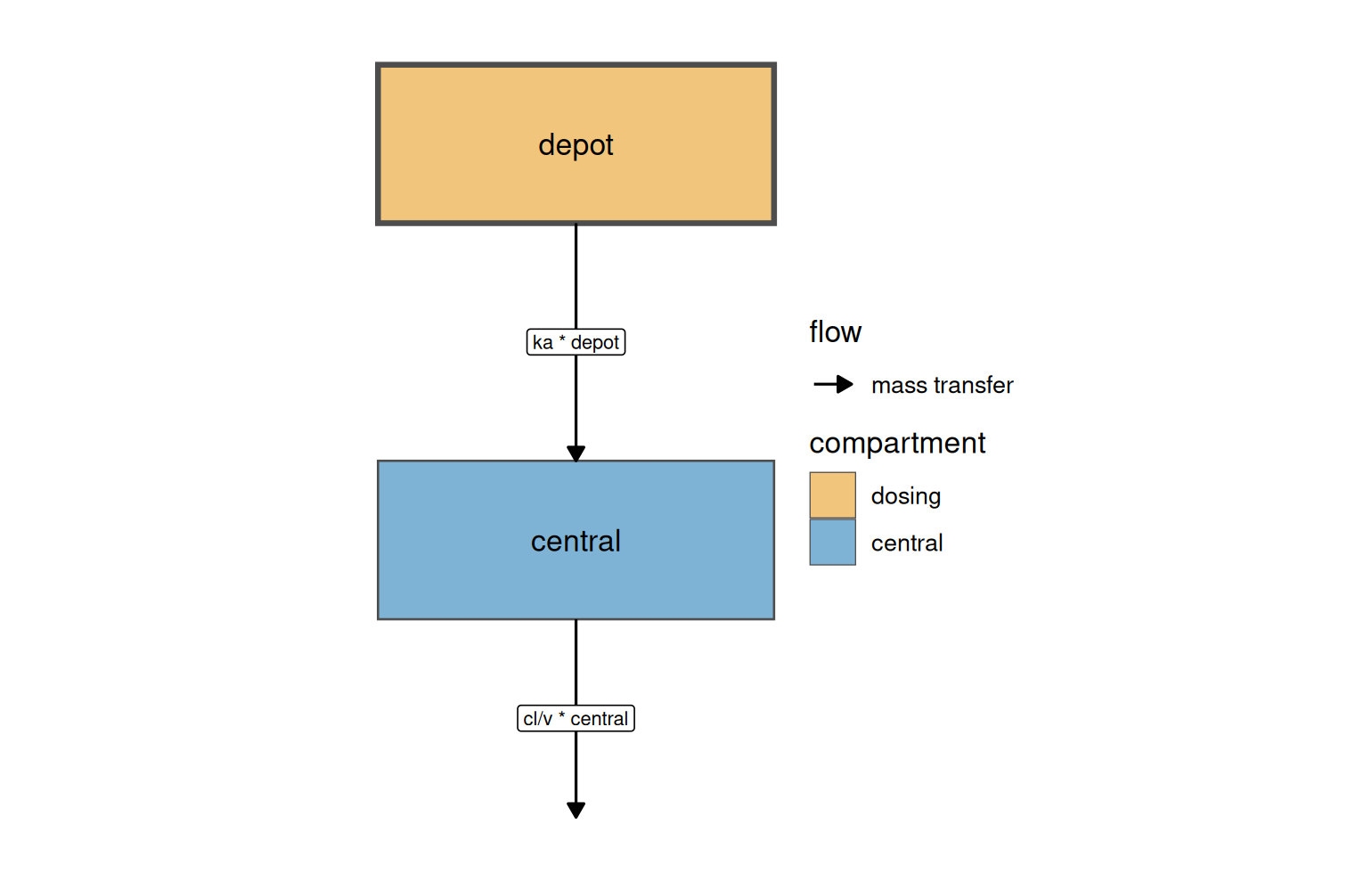
The model equations:
fit\[\begin{align*} {ka} & = \exp\left({tka}+{eta.ka}\right) \\ {cl} & = \exp\left({tcl}+{eta.cl}\right) \\ {v} & = \exp\left({tv}+{eta.v}\right) \\ \frac{d \: depot}{dt} & = -{ka} {\times} {depot} \\ \frac{d \: central}{dt} & = {ka} {\times} {depot}-\frac{{cl}}{{v}} {\times} {central} \\ {cp} & = \frac{{central}}{{v}} \\ {cp} & \sim add({add.sd}) \end{align*}\]
And, as usual, the parameter table:
fit$parFixedDf## Estimate SE %RSE Back-transformed CI Lower CI Upper
## tka 0.4609126 0.19152670 41.553800 1.5855203 1.0892912 2.3078077
## tcl 1.0117020 0.07894105 7.802796 2.7502781 2.3560357 3.2104903
## tv 3.4532980 0.04528458 1.311343 31.6044507 28.9202436 34.5377902
## add.sd 0.6968072 0.04718694 6.771879 0.6968072 0.6043225 0.7892919
## BSV(CV%) Shrink(SD)%
## tka 71.51577 -0.076938
## tcl 26.15932 3.893534
## tv 14.35110 11.210772
## add.sd NA NAThe diagram, the equations and the estimates all come from fit. If
the final model changes during review, re-knitting updates all three,
and the report cannot describe one model while its tables report
another. For regulatory work this also means that the QC of the
methods section is largely the QC of the code: there is no separate
hand-typed artifact to reconcile.
An end-to-end report: Word, HTML and PDF from one file
Here is the whole workflow as a single R Markdown report. It fits the
model, then writes a short methods and results section with the
diagram, the equations and the parameter table, and knits unchanged
to Word, HTML and PDF. Save it as model-report.Rmd (or download
the source):
---
title: "Theophylline population PK model"
output:
  bookdown::word_document2:
    number_sections: false
  bookdown::html_document2:
    number_sections: false
  bookdown::pdf_document2:
    number_sections: false
    toc: false
---

```{r setup, include = FALSE}
knitr::opts_chunk$set(echo = FALSE, message = FALSE, warning = FALSE,
                      fig.width = 6, fig.height = 4)
options(knitr.kable.NA = "")
library(nlmixr2)
library(nlmixr2plot)
library(nlmixr2extra)

# Model equations that work in Word, HTML and PDF.  Pandoc drops a bare
# align* environment when writing .docx, but converts display math
# ($$ ... $$) to native Word equations, so use an aligned block in
# display math for every format.  For Word, drop the alignment points
# (&, but not an escaped \& inside text) so the equations also display
# correctly in LibreOffice.
modelEquations <- function(x) {
  eq <- knitr::knit_print(x)
  if (knitr::pandoc_to("docx")) {
    eq <- gsub("(?<!\\\\)&", "", eq, perl = TRUE)
  }
  eq <- sub("\\begin{align*}", "$$\n\\begin{aligned}", eq, fixed = TRUE)
  eq <- sub("\\end{align*}", "\\end{aligned}\n$$", eq, fixed = TRUE)
  knitr::asis_output(eq)
}
```

```{r fit, include = FALSE}
one.cmt <- function() {
  ini({
    tka <- log(1.57)
    tcl <- log(2.72)
    tv <- log(31.5)
    eta.ka ~ 0.6
    eta.cl ~ 0.3
    eta.v ~ 0.1
    add.sd <- 0.7
  })
  model({
    ka <- exp(tka + eta.ka)
    cl <- exp(tcl + eta.cl)
    v <- exp(tv + eta.v)
    d/dt(depot) <- -ka * depot
    d/dt(central) <- ka * depot - cl / v * central
    cp <- central / v
    cp ~ add(add.sd)
  })
}
fit <- nlmixr2(one.cmt, nlmixr2data::theo_sd, est = "saem",
               control = saemControl(print = 0))
```

# Methods

Theophylline concentrations from `r length(unique(fit$ID))` subjects
were described by a one-compartment model with first-order absorption
(Figure \@ref(fig:diagram)), estimated with `r toupper(fit$est)` in nlmixr2.

```{r diagram, fig.cap = "Structure of the final model."}
modelDiagram(fit, engine = "ggplot2", labels = TRUE)
```

The model is defined by the following equations:

```{r equations}
modelEquations(fit)
```

# Results

The objective function value was `r round(fit$objf, 2)`.  Table
\@ref(tab:estimates) lists the final parameter estimates.

```{r estimates}
knitr::kable(fit$parFixedDf[, c("Back-transformed", "CI Lower",
                                "CI Upper", "%RSE", "BSV(CV%)")],
             digits = 3, caption = "Final parameter estimates.")
```
Two details make the same source work in every format:
- Equations. Pandoc silently drops a bare
\begin{align*}environment when it writes a.docxfile, so plainknit_print()output vanishes from Word documents. Wrapped as$$\begin{aligned} ... \end{aligned}$$it becomes a native, editable Word equation, and it still renders in HTML and PDF. For Word, the helper also drops the alignment points (&), so the Word equations are centered rather than aligned on the equals sign. Word itself handles aligned equations, but LibreOffice garbles them, and a report is often opened in more than one of them. ThemodelEquations()helper in the setup chunk does all of this, so one chunk serves all three formats. - Diagram.
engine = "ggplot2"gives a static image that every output format can embed. The interactive"DiagrammeR"widget only works in HTML. - Numbering. The
bookdownversions of the output formats (word_document2and friends) number the figure and table in every format, so\@ref(fig:diagram)and\@ref(tab:estimates)work in the text.
Rendering all three is one call:
rmarkdown::render("model-report.Rmd", output_format = "all")The PDF needs a LaTeX installation (for example
tinytex::install_tinytex()). Here are the results:
This is how the first page of each looks, Word on the left (opened in LibreOffice) and PDF on the right:
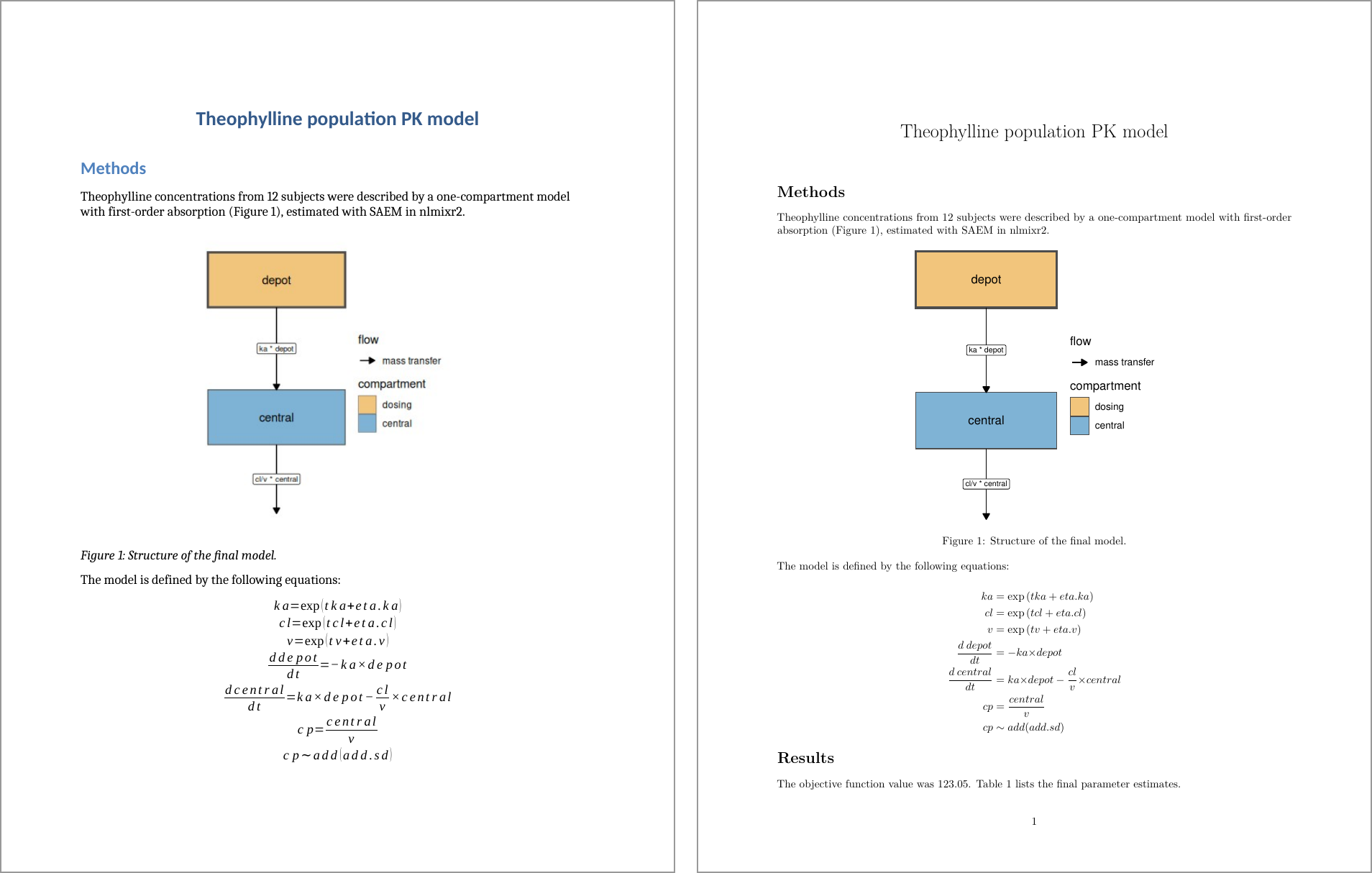
Your medical writers can open the Word version and edit the equations like any other Word equation. They can restyle the table too, and the diagram is regenerated from the model rather than redrawn. None of it has to be re-typed from the control stream.
A couple of notes for your own report templates:
- Variable names are the symbols. The equations use the names in
your model, so
eta.clstays \({eta.cl}\); it is not turned into \(\eta_{cl}\). Meaningful names in the code give readable equations in the report. - Swap in your own template. The report is ordinary R Markdown, so
a company Word template (
reference_docx) or a Quarto document works the same way. The only Word-specific piece is themodelEquations()wrapper.
Adding them to nlmixr2rpt reports
If your reports come from
nlmixr2rpt, which builds Word
and PowerPoint documents from a fit using your organization’s onbrand
templates, you get the diagram and the equations without doing
anything. From version 0.2.3 (currently the development version, on
its way to CRAN) the default report opens with the model: the diagram
from modelDiagram(), then the equations as native, editable Word and
PowerPoint math, ahead of the parameter table and the goodness-of-fit
figures nlmixr2rpt already produces. Until it reaches CRAN, install
it with remotes::install_github("nlmixr2/nlmixr2rpt").
Reporting a fit is the same call as before:
## Report the fit with the package's templates and default configuration
for (ext in c("docx", "pptx")) {
  obnd <- read_template(
    template = system.file(package = "nlmixr2rpt", "templates",
                           paste0("nlmixr_obnd_template.", ext)),
    mapping  = system.file(package = "nlmixr2rpt", "templates",
                           "nlmixr_obnd_template.yaml"))
  obnd <- report_fit(fit = fit, obnd = obnd)
  save_report(obnd, paste0("fit-report.", ext))
}
These are the first two pages of the Word report:
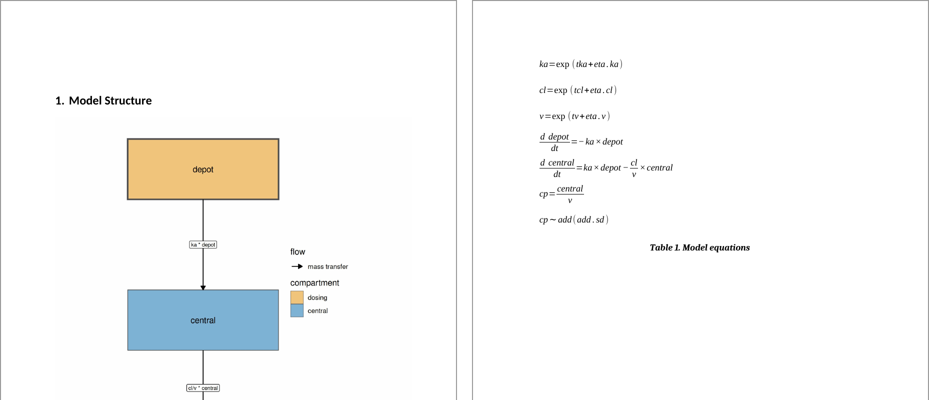
The equations come from a new function, gen_eqn_table(fit, obnd),
which puts one equation per row of a flextable and writes each row
as native math. With one equation per row there are no alignment
points, so Word and LibreOffice show the Word report the same way. If
you keep your own report configuration, add the diagram and the
equations to it with the same two entries the default now uses:
figures:
  model_diagram:
    cmd: |-
      p_res <- nlmixr2plot::modelDiagram(fit, engine = "ggplot2", labels = TRUE)
tables:
  model_equations:
    cmd: |-
      t_res <- list(ft = list(gen_eqn_table(fit, obnd)))
In PowerPoint the equations slide gets the same native math. There is no fallback image, though, so LibreOffice Impress and some other viewers show that slide blank.
Here are the generated Word report and PowerPoint deck, with the script that built them.
Try it
modelDiagram() and modelGraph() are in nlmixr2plot 5.2.0; the
knit_print() equations are in nlmixr2extra; and nlmixr2rpt 0.2.3
puts both in its Word and PowerPoint reports by default. Point them at the
model you are writing up this week and see how close they get you to
the figure and equations you would have drawn by hand. If a diagram
looks wrong, the issue
tracker is the place
to tell us – the model that trips up the parser is exactly the one we
want to see.