Adaptive dosing in rxode2

The idea in three lines

Decision logic goes inside the model({}) block, it runs at the times the solver visits, and when a condition is met you push a new event:

titrate <- function() {
  ini({
    ka <- 0.5
    cl <- 1
    v <- 10
  })
  model({
    d/dt(depot)   <- -ka*depot
    d/dt(central) <-  ka*depot - cl/v*central
    cp <- central/v
    # from day 1 on, top up if the daily check finds us below target

    # This is the code to say every 24 hours check to see if cp < 1,
    # then dose if needed
    if (t > 0 && t %% 24 == 0 && cp < 1) {
      bolus(50)
    }
  })
}

titrateSolve <- titrate |>
  rxSolve(et(amt = 100, time = 0) |> et(seq(0, 96, by = 1)))

ggplot(titrateSolve, aes(time, cp)) +
  geom_hline(yintercept = 1, linetype = 2, colour = "grey50") +
  geom_line(linewidth = 0.7, colour = "#2166ac") +
  theme_bw() +
  labs(x = "time (h)", y = "concentration",
       title = "Top up whenever the daily check finds us below target")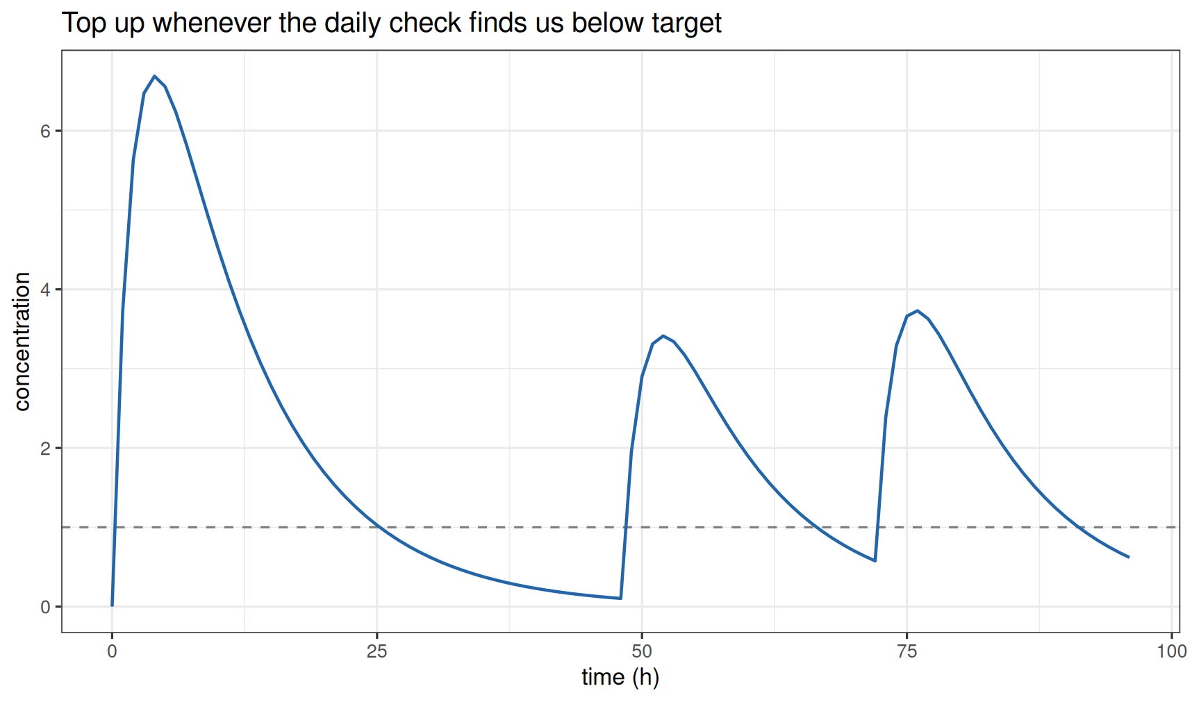

The helpers all push a standard NONMEM-style event, so there is nothing exotic downstream:

helper	evid	what it pushes
bolus()	1	a bolus dose, optionally with ii/addl/ss
infuse()	1	a fixed-rate infusion
infuseDur()	1	a fixed-duration infusion
reset()	3	a system reset
replace()	5	set a compartment to a value
multiply()	6	scale a compartment
phantom()	7	transit dosing bookkeeping (tad(), podo()) without mass
obs()	0	extra observation rows
evid_()	any	the low-level interface

Note that the condition is only tested at times the solver actually stops at; either the decision times have to be in the event table, or pinned with an mtime() assignment:

mtime(check48) <- 48        # note the assignment -- mtime(48) will not parse
if (t == check48 && cp < 1) {
  bolus(50)
}

A few things to keep in mind:

cp < 1 stays true almost always (except the first dose) so:

• alone it will fire almost every observation

• For it to be useful, it needs to be anchored to a visit (t == check48) or to a visit schedule, like every 24 hours (t %% 24 == 0).

This can be easy to get wrong. To prevent dosing at more times than you expect, you can use maxExtra to only add a specific number of doses per problem.

As a note, the t > 0 above matters too: at time zero cp is still 0, so without it the model will add a dose at time zero, even though the baseline dose is in the event table.

One last note, at the very end of the dosing if a new dose would be added, it won’t be shown in the observations since the model doesn’t check there or has no observations after the dose.

A model that needs this

One of the standard places where you need adaptive dosing is cancer treatment. For example, chemotherapy-induced neutropenia.

Friberg et al. (2002) described myelosuppression model under linear drug effect, three maturation transit compartments, and a rebound feedback term \((\mathrm{Circ}_0/\mathrm{Circ})^\gamma\). We took the estimates of docetaxel from Ozawa, Minami and Sato (2007), who fit a three-compartment PK model together with the Friberg neutropenia model in Japanese cancer patients:

doce <- function() {
  ini({
    cl <- 35.7 # L/h
    v1 <- 6.94 # L
    q2 <- 5.58 # L/h
    v2 <- 7.39 # L
    q3 <- 12.5 # L/h
    v3 <- 225 # L
    circ0 <- 5.05 # baseline neurtophil count *10^9/L
    mtt <- 113 # mean transit time (hr)
    gam <- 0.196 # shape
    slope <- 17.9 # mL / ug
  })
  model({
    ktr <- 4/mtt
    cp  <- central/v1

    d/dt(central) <- -(cl/v1)*central - (q2/v1)*central + (q2/v2)*periph1 -
                      (q3/v1)*central + (q3/v3)*periph2
    d/dt(periph1) <-  (q2/v1)*central - (q2/v2)*periph1
    d/dt(periph2) <-  (q3/v1)*central - (q3/v3)*periph2

    circS <- max(circ, 1e-4)
    d/dt(prol) <- ktr*prol*(1 - slope*cp)*(circ0/circS)^gam - ktr*prol
    d/dt(tr1)  <- ktr*(prol - tr1)
    d/dt(tr2)  <- ktr*(tr1  - tr2)
    d/dt(tr3)  <- ktr*(tr2  - tr3)
    d/dt(circ) <- ktr*(tr3  - circ)

    prol(0) <- circ0
    tr1(0) <- circ0
    tr2(0) <- circ0
    tr3(0) <- circ0
    circ(0) <- circ0

    anc <- circ # Absolute Neutrophil Count (ANC)
  })
}

Six cycles of docetaxel 100 mg/m^2 as a one-hour infusion every three weeks, in a 1.8 m^2 typical patient, is an ordinary event table:

bsa <- 1.8

fixedEv <- et(amt = 100*bsa, dur = 1, cmt = "central", ii = 21*24, addl = 5) |>
  et(seq(0, 126*24, by = 6))

typical <- rxSolve(doce, fixedEv)

ggplot(typical, aes(time/24, anc)) +
  geom_line(linewidth = 0.7) +
  geom_hline(yintercept = c(0.5, 1.5), linetype = 2, colour = "grey40") +
  theme_bw() +
  labs(x = "day", y = "ANC (10^9/L)",
       title = "Docetaxel 100 mg/m2 q3w, typical patient")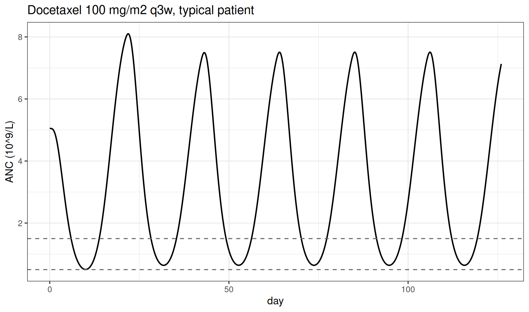

The nadir is 0.504 * 10^9/L on day 10, sitting just above the grade-4 line, and the count is back over 1.5 *10^9/L well before the next cycle: deep grade 3, no dose held, no dose cut.

The protocol only matters for the patients in the tail

As with all mixed effects models, for some patients it does matter. If we simulate 50 subjects on the same fixed schedule:

set.seed(20260909)
n <- 50
pop <- data.frame(
  id    = 1:n,
  cl    = 35.7*exp(rnorm(n, 0, 0.30)),
  slope = 17.9*exp(rnorm(n, 0, 0.35)),
  circ0 = 5.05*exp(rnorm(n, 0, 0.25)),
  mtt   =  113*exp(rnorm(n, 0, 0.20)))

popEv <- fixedEv |> et(id = 1:n)

popFixed <- rxSolve(doce, popEv, params = pop, returnType="data.frame")

doseDays <- (0:5)*21*24

popFixed |>
  filter(time %in% doseDays) |>
  summarise(`doses at ANC < 1.5` = sum(anc < 1.5), n = n())

##   doses at ANC < 1.5   n
## 1                  9 300

popFixed |>
  mutate(cycle = pmin(6, floor(time/504) + 1)) |>
  group_by(id, cycle) |>
  summarise(days = sum(anc < 0.5)*6/24, .groups = "drop") |>
  summarise(`cycles with >7 d grade 4` = sum(days > 7),
            `subjects affected` = n_distinct(id[days > 7]))

## # A tibble: 1 × 2
##   `cycles with >7 d grade 4` `subjects affected`
##                        <int>               <int>
## 1                         19                   4

Nine of the 300 planned doses land on a day when the neutrophil count is below 1500 cells/mm^3, and 19 cycles across four subjects sit at grade 4 for more than a week. The Taxotere label tells you what to do: don’t dose below 1500 cells/mm^3, and after febrile neutropenia or neutrophils under 500 cells/mm^3 for more than one week, step 100 mg/m^2 down to 75 mg/m^2, and then to 55 mg/m^2 if it happens again.

That is three coupled rules, and none of them can be written into et() because the answer depends on the solution.

Writing the label into the model

The protocol needs a memory: how long this cycle has been at grade 4, which dose level we are on, when the next cycle is due.

rxode2 can track this using sticky variables. Most left-hand-side variables in a model block are sticky: rather than being recomputed from nothing at each time point, they keep whatever value you last gave them, and they start out NA for each new individual. That gives the standard idiom – test for NA to initialise, then update in place:

if (is.na(level)) {
  level <- 1        # NA only at the first time point of each subject
}

Sticky variables make the protocol easy to read: updating one is an ordinary assignment.

Some things you need to keep in mind:

• The block runs once per record, not at internal solver steps

  • The weekly assessment fires with both t %% 168 == 0 and t >= nextDue. Then the nextDue assessment is incremented.

None of this touches the PK or the PD. To make sure that the model isn’t mis-typed, or copied or even so that if it i it will retain the dosing schedule, the best solution is to use model piping to appends the dosing protocol to doce and leave the model alone:

## Pipe the protocol onto the model we already have instead of writing
## the PK/PD out a second time.
##
## `auto = FALSE` keeps the auto selection of parameters off, so you
## can set the one new `bsa` parameter

doceProtocol <- doce |>
  model({
    ## --- protocol memory, in sticky variables ---------------------
    ## NA only at the first time point of each subject; after that
    ## these carry over from one time point to the next by themselves.
    if (is.na(level)) {
      level   <- 1        # 1 = 100, 2 = 75, 3 = 55 mg/m^2
      nextDue <- 21*24    # hour the next cycle is due
      dayLow  <- 0        # days at grade 4 since the last dose
      lastT   <- 0
    }
    dayLow <- dayLow + (anc < 0.5)*(time - lastT)/24
    lastT  <- time

    ## dose level for the cycle we are about to start
    newLevel <- level
    if (dayLow > 7) {
      newLevel <- level + 1
    }
    if (newLevel > 3) {
      newLevel <- 3
    }
    mgm2 <- 100
    if (newLevel > 1.5) {
      mgm2 <- 75
    }
    if (newLevel > 2.5) {
      mgm2 <- 55
    }
    doseMg  <- mgm2*bsa
    startMg <- 100*bsa

    ## --- cycle 1, then a weekly assessment ------------------------
    if (t == 0) {
      infuseDur(startMg, 1, central)
    }
    if (t > 0 && t < 126*24 && t %% 168 == 0 && t >= nextDue) {
      if (anc >= 1.5) {
        infuseDur(doseMg, 1, central)
        level   <- newLevel
        dayLow  <- 0
        nextDue <- t + 21*24
      } else {
        nextDue <- t + 7*24   # hold a week and reassess
      }
    }
  }, append = TRUE, auto = FALSE) |>
  ini(bsa <- 1.8)                     # m^2

Note that the amounts are assigned to plain variables first – infuseDur() wants a single symbol for amt, not an expression – and that the event table now carries no doses at all. Every dose is pushed by the model:

popAdapt <- rxSolve(doceProtocol,
                    et(seq(0, 126*24, by = 6)) |>
                      et(id = 1:n),
                    params = pop,
                    maxExtra = 500,
                    returnType="data.frame")

The sticky variable vignette has the other standard uses – running \(C_{max}\) and \(T_{max}\), time after dose, anything you would otherwise reach for a state to remember:

if (is.na(cMax)) {
  cMax <- 0
  tMax <- 0
}
if (cp > cMax) {
  cMax <- cp
  tMax <- time
}

One thing to keep in mind: dayLow is mildly grid-dependent.

One nice thing is the model’s decisions can be read straight back out of the solution, because nextDue advances by 504 h when a dose is given and 168 h when a cycle is held. It’s a sticky variable, so it changes on the same row where the decision was made — look behind, and the ANC you report is the one the protocol actually acted on.

Because nextDue moves by 504 h when a dose is given and 168 h when a cycle is held, the decisions the model made can be read straight back out of the solution. nextDue is a sticky variable, so it changes on the row the decision was taken – look behind, and the ANC you report is the one the protocol actually acted on.

decisions <- popAdapt |>
  group_by(id) |>
  arrange(id, time) |>
  mutate(step = c(0, diff(nextDue))) |>   # sticky: changes on the decision row
  ungroup()

given <- decisions |> filter(step == 504)
held  <- decisions |> filter(step == 168)

data.frame(what = c("doses given (cycles 2+)", "lowest ANC at a dose",
                    "cycles held", "subjects ever held"),
           value = c(nrow(given), round(min(given$anc), 2),
                     nrow(held), n_distinct(held$id)))

##                      what  value
## 1 doses given (cycles 2+) 249.00
## 2    lowest ANC at a dose   1.72
## 3             cycles held   4.00
## 4      subjects ever held   1.00

table(`mg/m2 given` = given$mgm2)

## mg/m2 given
##  55  75 100 
##   3  17 229

This can be handy in summarizing what happened in the simulated protocol.

In this case, no dose is now given below 1500 cells/mm^3 – the lowest count at any administration is 1.72 × 10^9/L – and twenty of the 249 later doses are given at a reduced level.

Counting 21-day windows the same way as before, the number spent at grade 4 for more than a week falls from 19 to five:

decisions |>
  mutate(window = pmin(6, floor(time/504) + 1)) |>
  group_by(id, window) |>
  summarise(days = sum(anc < 0.5)*6/24, .groups = "drop") |>
  summarise(`windows with >7 d grade 4` = sum(days > 7))

## # A tibble: 1 × 1
##   `windows with >7 d grade 4`
##                         <int>
## 1                           5

The five patients it happened to

Four subjects were dose-reduced and one had cycles held. Two of them are worth looking at.

Subject 47 is slow to recover (mean transit time 203 h): under the fixed schedule the count is still between 1.1 and 1.5 × 10^9/L on every planned dosing day from cycle 2 onwards. Subject 24 clears docetaxel slowly (CL 20.3 L/h) and is sensitive to it (slope 31.7 mL/µg), spends over nine days at grade 4 in cycle 1 and is still over the line two cycles after the first reduction – the only subject in the trial to walk the whole 100 → 75 → 55 ladder.

ids <- c(24, 47)

lab <- c("24" = "subject 24 -- dose reduced 100 -> 75 -> 55 mg/m2",
         "47" = "subject 47 -- each cycle delayed one week")

bind_rows(
  popFixed |> filter(id %in% ids) |> mutate(schedule = "fixed q3w"),
  popAdapt |> filter(id %in% ids) |> mutate(schedule = "label protocol")) |>
  mutate(who = lab[as.character(id)]) |>
  ggplot(aes(time/24, anc, colour = schedule)) +
  geom_hline(yintercept = c(0.5, 1.5), linetype = 2, colour = "grey50") +
  geom_line(linewidth = 0.7) +
  facet_wrap(~who, ncol = 1, scales = "free_y") +
  scale_colour_manual(values = c("fixed q3w" = "grey45",
                                 "label protocol" = "#2166ac")) +
  labs(x = "day", y = "ANC (10^9/L)", colour = NULL)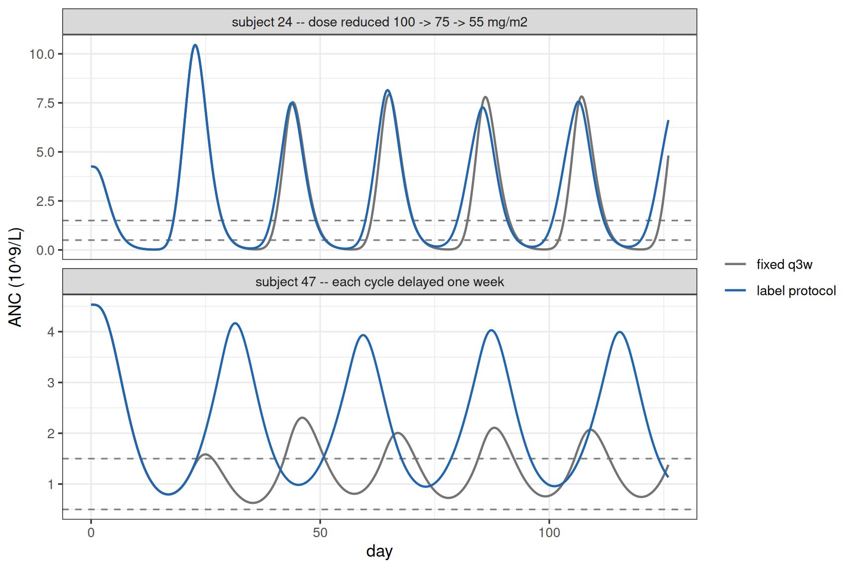

The two panels show the two things a protocol can change: when and how-much.

Subject 47 illustrates when: the blue curve’s cycles are 28 days apart instead of 21.

Subject 24 is about how much – reducing the dose does not lift the nadir, it shortens the time spent there. Its own cycles go from 9.2 days at grade 4 before the first reduction to 5.8 after the second; s

Either way, the grey and blue curves are the same model, the same parameters and the same 126 days. The only difference is that in the blue one the event history was written by the solver.

Notes from actually using it

A few things that will save you an some time:

• Decision times must exist. The logic runs at output times. If the assessment is not in et(), pin it with mtime().

• Guard against re-triggering. anc >= 1.5 is true for weeks. Anchoring on t %% 168 == 0 is what turns a standing condition into a single decision.

• Bookkeeping belongs in sticky variables, not states. Counters, dose levels and “when is the next visit” carry over from one time point to the next on their own, you could use states instead but it takes more time to solve the system. is.na() is how you initialise them.

• Currently the dose amt wants a symbol. Compute doseMg <- mgm2*bsa on its own line; infuseDur(mgm2*bsa, ...) will not parse. In the future this may change.

• Set maxExtra. It is a cheap way to find out that your condition fires 4000 times instead of six.

• At the last output time the event is dropped but the sticky assignment is not. There is no row left to put a pushed event in, so the dose never happens – but nextDue and dayLow are ordinary assignments and go through anyway.

• Reading decisions back out of the state vector only works if the decision times are on the grid. filter(step == 504) is exact equality on a float; it survives here because 168 and 504 land exactly on a 6 h grid. Solve on by = 5 and the summary silently reports zero doses rather than erroring.

• linCmt() works too, and odeToLin() will convert a linear ODE model that uses adaptive dosing into the analytic form – worth it when you are running that kind of model over many trial designs. It cannot help the example above, whose PD is nonlinear.

Where to read more

The adaptive dosing vignette is the reference: every helper, the evid_() low-level interface, phantom dosing for transit models, adaptive sampling with obs(), and the linCmt() and odeToLin() story.

The obvious next step is that these protocol rules are now part of the model, which means they can be part of a trial simulation – compare two dose-modification tables, or ask what a different assessment schedule would have bought you, without leaving rxode2.

References

• Friberg LE, Henningsson A, Maas H, Nguyen L, Karlsson MO. Model of chemotherapy-induced myelosuppression with parameter consistency across drugs. J Clin Oncol. 2002;20(24):4713-4721.
• Ozawa K, Minami H, Sato H. Population pharmacokinetic and pharmacodynamic analysis for time courses of docetaxel-induced neutropenia in Japanese cancer patients. Cancer Sci. 2007;98(12):1985-1992.
• TAXOTERE (docetaxel) prescribing information, Sanofi-Aventis.