Survival Analysis with nlmixr2
By Justin Wilkins and the nlmixr2 Development Team in nlmixr2
May 28, 2026
Introduction
Survival or time-to-event (TTE) analysis models when something happens, not just whether it happens. The endpoint might be time to tumour progression, time to an adverse event, or time to treatment discontinuation, for instance. In this post we’ll illustrate how to fit parametric TTE models in nlmixr2 using its custom log-likelihood interface.
For the purposes of this post, we’re going to simulate a two-arm randomised trial from a known Gompertz model, then recover the parameters with nlmixr2. This is cheating, obviously, but since we’ll know what the truth is, we’ll be able to directly assess how well the model does in recovering the parameters.
It’s worth mentioning that the kind of analysis we show here can be performed using other R packages, like flexsurv, probably in a more straightforward way, but where things get interesting is with more complex models. We only show the basics here, but the potential is endless…
Simulated Dataset
We are going to generate 300 patients (150 per arm) from a Gompertz proportional-hazards model with increasing hazard (\(\gamma > 0\)) and a 50% drug-induced hazard reduction (HR = 0.5).
\[h(t \mid \text{test\_trt}) = \underbrace{\alpha \, e^{\gamma t}}_{\text{baseline Gompertz}} \cdot \exp(\beta \cdot \text{test\_trt})\]
| Parameter | True value | Interpretation |
|---|---|---|
| \(\alpha\) | 0.002 /day | Initial hazard (placebo) |
| \(\gamma\) | 0.005 /day | Hazard growth rate; \(\gamma>0\) → increasing risk |
| \(\beta\) | \(\log(0.5) \approx -0.693\) | Log hazard ratio, drug vs. placebo |
We’ll use a universal cutoff at 365 days. We can use the closed-form Gompertz inverse-CDF for simulation:
n_arm       <- 150
true_alpha  <- 0.002
true_gamma  <- 0.005
true_log_hr <- log(0.5)
maxt        <- 365

n_total  <- 2L * n_arm
test_trt <- rep(0L:1L, each = n_arm)   # 0 = placebo, 1 = drug

u       <- runif(n_total)
hr_vec  <- exp(true_log_hr * test_trt)
# Gompertz inverse-CDF: t = log(1 + gamma*(-log U)/(alpha*hr)) / gamma
t_event <- log(1 + true_gamma * (-log(u)) / (true_alpha * hr_vec)) / true_gamma

tte_sim <- data.frame(
  id       = seq_len(n_total),
  time     = pmin(t_event, maxt),
  event    = as.integer(t_event <= maxt),
  test_trt = test_trt,
  dv       = pmin(t_event, maxt),
  evid     = 0L
)

cat(sprintf(
  "%d patients | Placebo: %d events (%.0f%%) | Drug: %d events (%.0f%%)\n",
  nrow(tte_sim),
  sum(tte_sim$event[tte_sim$test_trt == 0]),
  100 * mean(tte_sim$event[tte_sim$test_trt == 0]),
  sum(tte_sim$event[tte_sim$test_trt == 1]),
  100 * mean(tte_sim$event[tte_sim$test_trt == 1])
))
## 300 patients | Placebo: 134 events (89%) | Drug: 91 events (61%)The increasing hazard means events become more frequent late in follow-up. The drug-treatment arm retains more survivors throughout.
Exploratory Analysis
Plotting the data is something everyone should always do first.
tte_sim$trt_label <- factor(tte_sim$test_trt, levels = 0:1,
                             labels = c("Placebo", "Drug"))
km_fit <- survfit(Surv(time, event) ~ trt_label, data = tte_sim)

ggsurvplot(
  km_fit, data = tte_sim,
  palette      = c("steelblue", "firebrick"),
  legend.labs  = c("Placebo", "Drug"),
  legend.title = "Arm",
  xlab = "Days", ylab = "Survival probability",
  title   = "Kaplan-Meier curves by treatment arm (simulated Gompertz data)",
  conf.int = TRUE, ggtheme = theme_bw()
)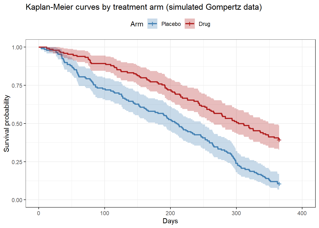
The two arms separate clearly (by design, of course). Note the acceleration in event rate late in follow-up — a signature of the increasing (\(\gamma > 0\)) Gompertz hazard that a typical exponential model cannot capture accurately.
Hazard shape exploration
Before choosing a parametric form, we overlay several distributions against a
kernel density hazard estimate and compare AICs. The plot_hazard helper below
fits six standard distributions and two cubic-spline models via flexsurv.
plot_hazard(dat = tte_sim, stime = "time", evt = "event")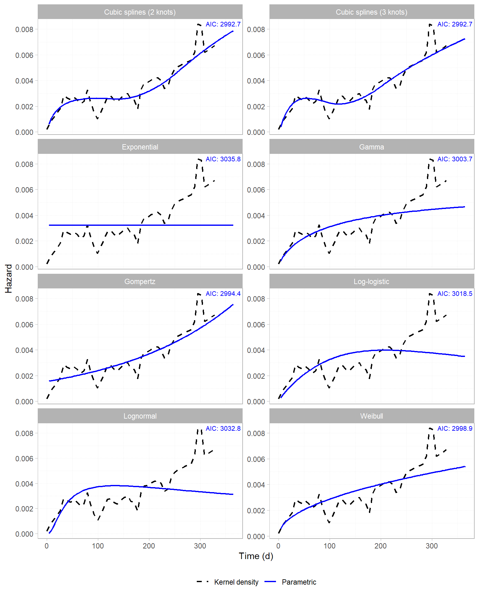
The Gompertz panel tracks the kernel density closely, as expected from a correctly-specified model. The exponential panel (constant hazard) clearly doesn’t work here, although some of the other alternatives do reasonably well.
Model 1 — Exponential (Constant Hazard)
The exponential model assumes constant hazard over time. We know this is the wrong model, but it’s a handy baseline for comparison. The drug effect is represented by \(trt_i\), which is 0 (placebo) or 1 (treatment):
\[h_i(t) = h_0 \exp(\beta \cdot trt_i)\]
The log-likelihood contribution per patient is:
\[\ell_i = \delta_i \log h_i - H_i(t_i) = \delta_i \log h_i - h_i \, t_i\]
where \(\delta_i = 1\) for an event and \(0\) for a censored observation.
In nlmixr2 we can write this via the ll() interface:
exp_model <- function() {
  ini({
    log_h0      <- log(0.004)
    test_log_hr <- -0.1
  })
  model({
    log_h  <- log_h0 + test_log_hr * test_trt
    h      <- exp(log_h)
    H      <- h * time
    tte_ll <- event * log_h - H
    ll(tte) ~ tte_ll
  })
}

fit_exp <- nlmixr(exp_model, tte_sim, est = "bobyqa",
                  control = bobyqaControl(print = 0))
## [====|====|====|====|====|====|====|====|====|====] 0:00:00## [====|====|====|====|====|====|====|====|====|====] 0:00:00## |-----+---------------+-----------+-----------|fit_exp$parFixedDf## Estimate SE %RSE Back-transformed CI Lower
## log_h0 -5.4143350 0.1727737 3.191042 -5.4143350 -5.752965
## test_log_hr -0.6717797 0.2716741 40.440951 -0.6717797 -1.204251
## CI Upper BSV(SD) Shrink(SD)%
## log_h0 -5.0757048 NA NA
## test_log_hr -0.1393082 NA NASo far so good.
Model 2 — Gompertz (Increasing Hazard)
The Gompertz model adds a shape parameter \(\gamma\) governing the rate of hazard change. With \(\gamma > 0\) the hazard increases exponentially, as we saw in the plot comparing hazard functions above.
\[h_i(t) = \alpha \, e^{\gamma t} \exp(\beta \cdot trt_i) \qquad H_i(t) = \frac{\alpha}{\gamma}\bigl(e^{\gamma t}-1\bigr) \exp(\beta \cdot trt_i)\]
Important: both \(\alpha\) and \(\gamma\) are log-transformed in the ini() block so that
all three estimated parameters live on a similar numerical scale. This avoids
potential conditioning problems that arise when the bobyqa estimation method has to simultaneously adjust parameters of magnitude \(\sim\!10^{-3}\) and \(\sim\!10^{0}\), which can lead to the model getting stuck in local minima.
In the model below, we’ve added a drug effect using test_log_hr.
gompertz_model <- function() {
  ini({
    log_alpha   <- log(0.003)
    log_gamma   <- log(0.003)   # gamma = exp(log_gamma) > 0 enforced
    test_log_hr <- -0.5         # informed by KM: ~40-50% separation visible
  })
  model({
    alpha  <- exp(log_alpha)
    gamma  <- exp(log_gamma)
    h      <- alpha * exp(gamma * time) * exp(test_log_hr * test_trt)
    H      <- (alpha / gamma) * (exp(gamma * time) - 1) * exp(test_log_hr * test_trt)
    tte_ll <- event * log(h) - H
    ll(tte) ~ tte_ll
  })
}

fit_gompertz <- nlmixr(gompertz_model, tte_sim, est = "bobyqa",
                       control = bobyqaControl(print = 0))
## |-----+---------------+-----------+-----------+-----------|fit_gompertz$parFixedDf## Estimate SE %RSE Back-transformed CI Lower
## log_alpha -6.1731625 0.2951631 4.781392 0.002084633 0.001168924
## log_gamma -5.3212965 0.2744153 5.156925 0.004886414 0.002853695
## test_log_hr -0.7986951 0.2743202 34.346044 -0.798695075 -1.336352718
## CI Upper BSV(SD) Shrink(SD)%
## log_alpha 0.003717687 NA NA
## log_gamma 0.008367062 NA NA
## test_log_hr -0.261037432 NA NAtheta_g <- fit_gompertz$theta
kable(
data.frame(
Parameter = c("alpha (/day)", "gamma (/day)", "HR (drug vs. placebo)"),
True = c(true_alpha, true_gamma, exp(true_log_hr)),
Estimated = round(c(exp(theta_g["log_alpha"]),
exp(theta_g["log_gamma"]),
exp(theta_g["test_log_hr"])), 4),
Interpretation = c(
"Initial hazard at t = 0, placebo arm",
"Hazard growth rate; >0 confirms increasing risk",
"Instantaneous hazard ratio, drug vs. placebo"
)
),
digits = 4,
caption = "Gompertz parameter recovery: true vs. estimated values"
)| Parameter | True | Estimated | Interpretation | |
|---|---|---|---|---|
| log_alpha | alpha (/day) | 0.002 | 0.0021 | Initial hazard at t = 0, placebo arm |
| log_gamma | gamma (/day) | 0.005 | 0.0049 | Hazard growth rate; >0 confirms increasing risk |
| test_log_hr | HR (drug vs. placebo) | 0.500 | 0.4499 | Instantaneous hazard ratio, drug vs. placebo |
The model recovers \(\alpha\) and \(\gamma\) closely. The estimated HR is in the right direction and magnitude; there’s a bit of deviation from the true 0.5, reflecting the limitations of this kind of data.
As we alluded to above, starting estimates matter. bobyqa is a trust-region optimizer with no built-in multi-start, so it can get stuck if the initial values are far from the truth. If the parameter estimates look suspicious, try perturbing the ini() values, or increase npt in bobyqaControl() — e.g. npt = 7 (Powell’s recommended \(2n+1\) for \(n = 3\) parameters) gives the quadratic approximation more
interpolation points and a better chance of finding the global optimum. For
difficult problems, running from a small grid of starting values and keeping
the fit with the lowest objective function value is probably the most robust approach.
Model Comparison
aic_table <- AIC(fit_exp, fit_gompertz) %>%
  as.data.frame() %>%
  tibble::rownames_to_column("Model") %>%
  mutate(
    Model = c("Exponential", "Gompertz"),
    m2LL  = round(c(-2 * logLik(fit_exp), -2 * logLik(fit_gompertz)), 2)
  )

kable(aic_table, digits = 2,
caption = "AIC and -2 log-likelihood: exponential vs. Gompertz")| Model | df | AIC | m2LL |
|---|---|---|---|
| Exponential | 2 | 3012.71 | 3008.71 |
| Gompertz | 3 | 2961.64 | 2955.64 |
The Gompertz fit is unambiguously the best. Since this is a simulated example, it would be weird if it wasn’t!
theta_e <- fit_exp$theta
h0_exp  <- exp(theta_e["log_h0"])
alpha_g <- exp(theta_g["log_alpha"])
gamma_g <- exp(theta_g["log_gamma"])

t_grid <- seq(0, maxt, length.out = 400)

exp_surv      <- function(t)     exp(-h0_exp * t)
gompertz_surv <- function(t, hr) exp(-(alpha_g / gamma_g) * (exp(gamma_g * t) - 1) * hr)

model_pred_df <- bind_rows(
  data.frame(time = t_grid, survival = exp_surv(t_grid),         model = "Exponential"),
  data.frame(time = t_grid, survival = gompertz_surv(t_grid, 1), model = "Gompertz")
)

km_plac    <- survfit(Surv(time, event) ~ 1, data = filter(tte_sim, test_trt == 0))
km_plac_df <- data.frame(time     = c(0, km_plac$time),
                          survival = c(1, km_plac$surv),
                          model    = "Kaplan-Meier")

ggplot() +
  geom_step(data = km_plac_df,    aes(time, survival, color = model), linewidth = 0.8) +
  geom_line(data = model_pred_df, aes(time, survival, color = model), linewidth = 1) +
  scale_color_manual(values = c("Kaplan-Meier" = "black",
                                "Exponential"  = "steelblue",
                                "Gompertz"     = "firebrick")) +
  labs(x = "Days", y = "Survival probability",
       title = "Exponential vs. Gompertz model fit (placebo arm)", color = NULL) +
  coord_cartesian(ylim = c(0, 1)) +
  theme_bw() + theme(legend.position = "bottom")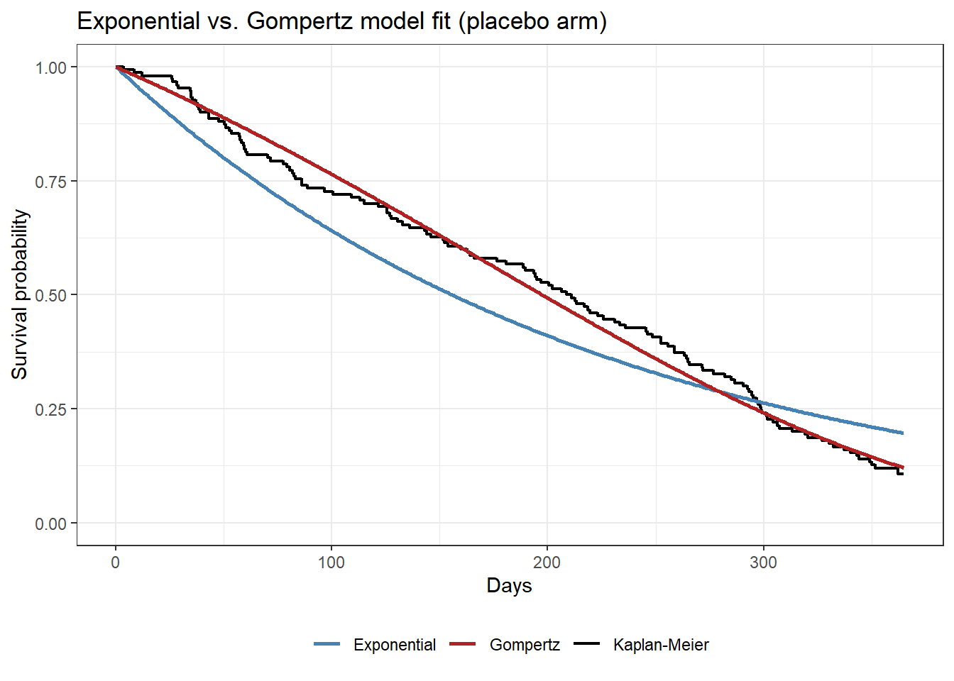
The ΔAIC of ~71 units and the plot make the same point: the exponential model starts too high early and ends too high late, because it cannot accommodate the accelerating risk. The Gompertz curve, by contrast, is much close to the Kaplan-Meier curve.
Predicted Survival Curves vs. Observed KM
hr_drug <- exp(theta_g["test_log_hr"])

pred_df <- bind_rows(
  data.frame(time = t_grid, survival = gompertz_surv(t_grid, 1),       arm = "Placebo (predicted)"),
  data.frame(time = t_grid, survival = gompertz_surv(t_grid, hr_drug), arm = "Drug (predicted)")
)

km_arms <- lapply(c(0, 1), function(d) {
  label <- if (d == 0) "Placebo" else "Drug"
  fit   <- survfit(Surv(time, event) ~ 1, data = filter(tte_sim, test_trt == d))
  data.frame(time = c(0, fit$time), survival = c(1, fit$surv),
             arm = paste0(label, " (KM)"))
})
km_df2 <- bind_rows(km_arms)

cols <- c("Placebo (KM)"      = "steelblue", "Placebo (predicted)" = "steelblue",
          "Drug (KM)"         = "firebrick", "Drug (predicted)"    = "firebrick")

ggplot() +
  geom_step(data = km_df2,  aes(time, survival, color = arm), linewidth = 0.8) +
  geom_line(data = pred_df, aes(time, survival, color = arm),
            linewidth = 1, linetype = "dashed") +
  scale_color_manual(values = cols) +
  labs(x = "Days", y = "Survival probability",
       title = "Gompertz model vs. Kaplan-Meier by arm (simulated data)",
       color = NULL) +
  coord_cartesian(ylim = c(0, 1)) +
  theme_bw() + theme(legend.position = "bottom")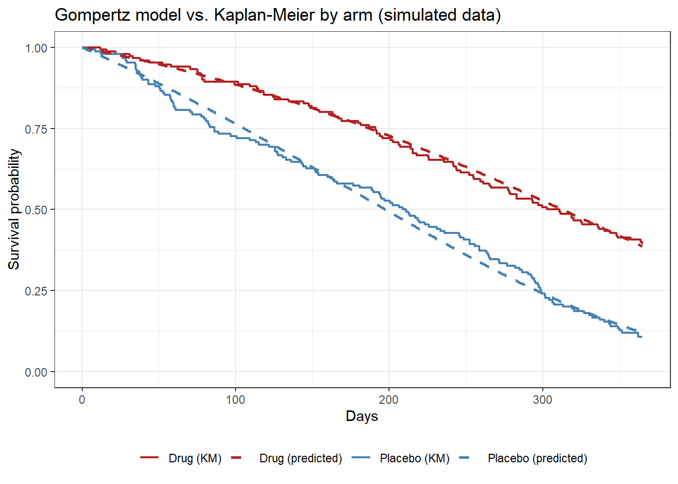
Dashed lines are Gompertz predictions; solid steps are the Kaplan-Meier estimates. The predicted curves track both arms closely across the full follow-up period.
A TTE VPC
We can use the vpc package to generate a TTE visual predictive check (VPC)…
n_vpc_sim <- 200
set.seed(8675)

vpc_obs <- tte_sim %>%
  transmute(id = id, t = time, dv = event, trt = trt_label)

vpc_sim <- bind_rows(
  lapply(seq_len(n_vpc_sim), function(s) {
    u      <- runif(nrow(tte_sim))
    hr_vec <- exp(theta_g["test_log_hr"] * tte_sim$test_trt)
    t_evt  <- log(1 + gamma_g * (-log(u)) / (alpha_g * hr_vec)) / gamma_g
    data.frame(
      sim = s,
      id  = tte_sim$id,
      t   = pmin(t_evt, maxt),
      dv  = as.integer(t_evt <= maxt),
      trt = tte_sim$trt_label
    )
  })
)

suppressMessages(suppressWarnings(
  vpc::vpc_tte(
    obs      = vpc_obs,
    sim      = vpc_sim,
    obs_cols = list(id = "id", idv = "t", dv = "dv"),
    sim_cols = list(id = "id", idv = "t", dv = "dv", sim = "sim"),
    stratify = "trt",
    plot     = FALSE,
    as_percentage = FALSE,
    xlab  = "Days",
    ylab  = "Survival probability",
    title = "Gompertz TTE VPC by treatment arm"
  )
))
## ================================================================================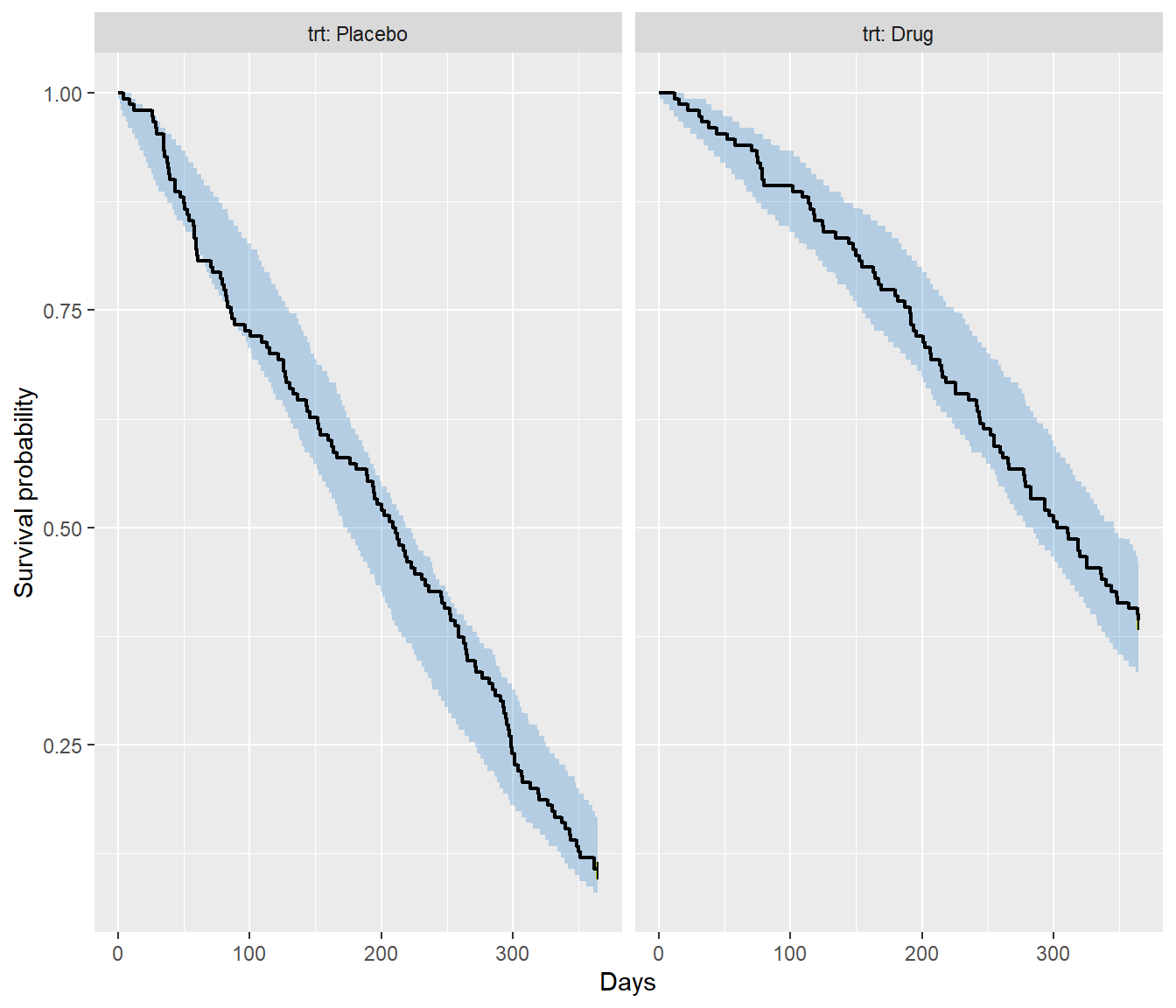
The shaded band is the 95% prediction interval of the simulated survival curves across the 200 replicates, while the solid line is the observed Kaplan-Meier for placebo and active treatment arms. Both arms sit within their bands throughout follow-up, confirming that the fitted model is adequately reproducing the observed data.
Wrapping it up
So that’s how to fit parametric TTE models in nlmixr2 using
the custom log-likelihood interface (ll(tte) ~ tte_ll). To recap, the workflow is:
- Wrangle data into
id / time / dv / evid / eventformat. - Define hazard \(h\) and cumulative hazard \(H\) in the
model()block. - Fit with
nlmixr()usingbobyqa(no symbolic gradients required). - Log-transform shape parameters with potentially small values to keep all parameters on a comparable scale for the optimizer.
The Gompertz model recovered the known simulation parameters closely in this synthetic example. We can extend the same structure naturally to exposure-driven TTE models and repeated time-to-event endpoints. Watch this space!
- Posted on:
- May 28, 2026
- Length:
- 10 minute read, 2054 words
- Categories:
- nlmixr2
- Tags:
- time-to-event survival tutorial
- See Also: