Fitting PK/PD models to published data with admixr2
By H. van de Beek in nlmixr2
July 2, 2026
Usually, pharmacometric modelling starts with a dataset with individual patient data: one row per observation, in a software-ready format. To model these data, you would first need to get access to the data, which means data-sharing agreements, trial access, or in-house studies. This process is often slow or even not possible due to privacy or competition. However, researchers do publish their model and sometimes summary metrics.
The published reports do contain useful information. A publication of a PK study often contains mean concentration-time profiles with standard deviations, and the PK model structure and estimates. None of these data are individual patient data - but they can still be used for modelling, using aggregate data modelling.
admixr2 is an R package that fits pharmacometric models directly to these aggregate summaries or published models. The package integrates the methodology directly into the nlmixr2/rxode2 ecosystem: you write models using familiar syntax: ini() / model(). To use this method, you call nlmixr2() with est = "adfo", est = "admc", est = "adgh", or est = "adirmc".
This post covers the two main ways published data can be modelled using admixr2, and shows how to combine multiple sets of summary data in a single joint fit.
What admixr2 fits to
admixr2 can be used to model aggregate data, either from published time-profiles or from published models. However, both are based on two quantities per study:
- E - the observed mean drug concentration vector at the measurement times, \(\bar{y} \in \mathbb{R}^T\).
- V - the observed (co)variance matrix, \(S \in \mathbb{R}^{T \times T}\).
Given a mixed-effects model predicting population mean \(\mu\) and covariance \(V_\text{pred}\), we can calculate the aggregate log-likelihood incorporating the study sample size \(n\). The result is the likelihood for the sample mean and covariance: it rewards a model whose predicted population distribution matches both the average profile and the spread and correlation structure in the data.
So for modelling aggregate data, you specify E, V, times and n once per study and then call nlmixr2() exactly as you would for individual-level fitting. The rest - optimizer, standard errors, AIC, diagnostic plots - works similar to nlmixr2.
Usecase 1: digitized mean ± SD from the literature
Say you found two published studies of a hypothetical intravenous compound. One used a 100 mg dose in 40 subjects, the other 200 mg in 35 subjects. Both report mean concentrations and standard deviations at five time points, either in a table or in figures that you digitized with a plotdigitizer.
You have means and SDs - not the full covariance matrix. admixr2 handles this using method = "var", which uses only the diagonal of V (the marginal variances) in the likelihood. Just pass a diagonal matrix or a variance vector:
library(rxode2)
library(nlmixr2)
library(admixr2)
library(ggplot2)

times_measured <- c(0.5, 1, 2, 4, 8)

# Study A: 100 mg IV bolus, n = 40
# Values represent typical digitized output (mean, SD) -> SD^2 on the diagonal
study_a <- list(
  E     = c(2.33, 1.84, 1.23, 0.51, 0.09),   # mg/L
  V     = diag(c(0.341, 0.212, 0.095, 0.016, 0.0005)),  # SD^2
  n     = 40L,
  times = times_measured,
  ev    = et(amt = 100)
)

# Study B: 200 mg IV bolus, n = 35
study_b <- list(
  E     = c(4.57, 3.77, 2.41, 1.04, 0.18),
  V     = diag(c(1.009, 0.688, 0.281, 0.052, 0.0016)),
  n     = 35L,
  times = times_measured,
  ev    = et(amt = 200)
)
Plotting the two digitized profiles shows the summary data we are working with - a mean curve and a marginal spread at each timepoint, with no access to the underlying individual trajectories:
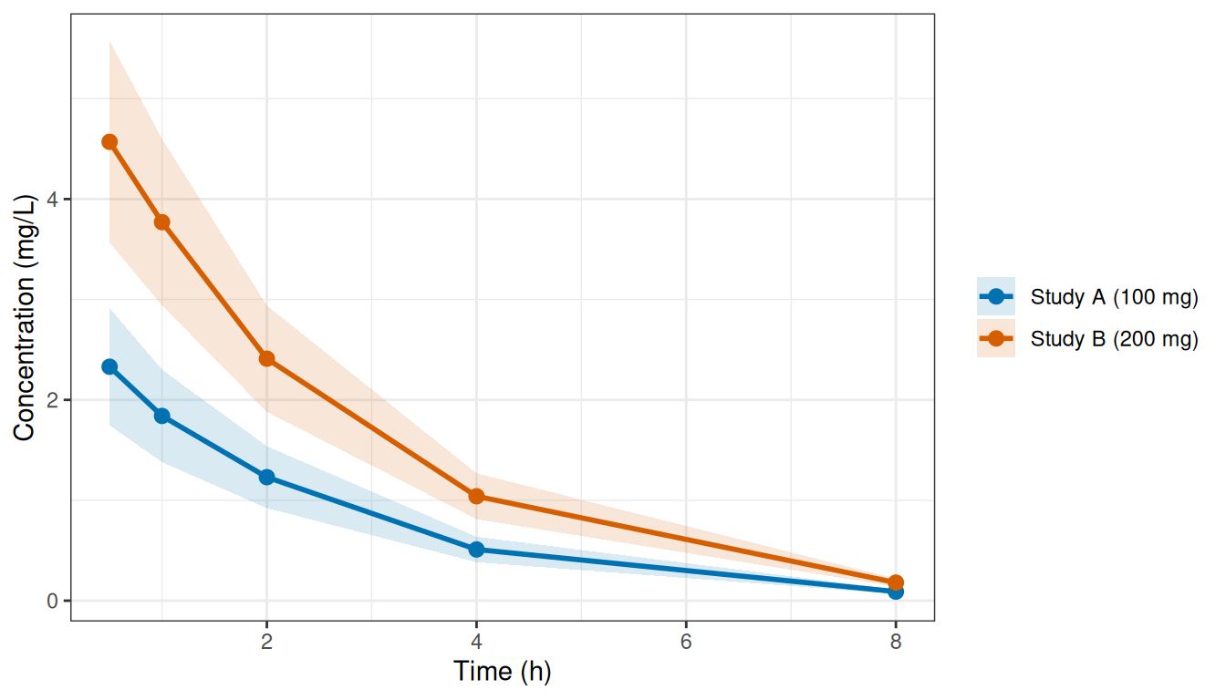
Figure 1: Digitized mean ± 1 SD for the two published IV studies.
The analysis model is a standard one-compartment IV model written in nlmixr2 syntax:
pk_1cmt_iv <- function() {
  ini({
    tcl    <- log(10)       # log CL (L/h) -- starting value
    tv     <- log(40)       # log V (L)
    eta.cl ~ 0.12
    eta.v  ~ 0.06
    add.err <- c(0, 0.15)
  })
  model({
    cl <- exp(tcl + eta.cl)
    v  <- exp(tv  + eta.v)
    d/dt(centr) <- -(cl / v) * centr
    cp <- centr / v
    cp ~ add(add.err)
  })
}
Fitting is a single nlmixr2() call with for example est = "admc", the estimator that uses simulation to estimate the IIV distribution. The studies argument names the two studies; admData() is a placeholder dataset required by nlmixr2 in the background, but it carries no actual observations:
fit_lit <- nlmixr2(
  pk_1cmt_iv, admData(), est = "admc",
  control = admControl(
    studies   = list(study_a = study_a, study_b = study_b),
    n_sim     = 2000L,
    covMethod = "r"
  )
)
Printing the fit gives the standard nlmixr2 summary - objective function, information criteria, and the population parameters with their estimates back-transformed to the natural scale (here CL and V):
print(fit_lit)## ── nlmixr² admc ──
##
## OBJF AIC BIC Log-likelihood
## admc -484.4386 -474.4386 -454.804 242.2193
##
## ── Time (sec fit_lit$time): ──
##
## optimize covariance elapsed
## 1 5.191 2.167 7.358
##
## ── Population Parameters (fit_lit$parFixed or fit_lit$parFixedDf): ──
##
## Est. SE %RSE Back-transformed(95%CI) BSV(CV%) Shrink(SD)%
## tcl 2.717 0.01449 0.5332 15.14 (14.71, 15.57) 18.93
## tv 3.49 0.02289 0.6559 32.79 (31.35, 34.3) 30.21
## add.err 0.01231 0.01231
##
## Covariance Type (fit_lit$covMethod): r
## No correlations in between subject variability (BSV) matrix
## Full BSV covariance (fit_lit$omega)
## or correlation (fit_lit$omegaR; diagonals=SDs)
## Distribution stats (mean/skewness/kurtosis/p-value) available in $shrink
## Censoring (fit_lit$censInformation): No censoring
## Minimization message (fit_lit$message):
## NLOPT_XTOL_REACHED: Optimization stopped because xtol_rel or xtol_abs (above) was reached.
The resulting fit_lit is a standard nlmixr2 fit object: AIC(fit_lit), logLik(fit_lit), plot(fit_lit) all work as expected.
The plot() method also takes a which argument to select diagnostics - "mean", "cov", "nll", or "par". With which = "mean" it overlays the fitted population mean (with predicted spread) on the observed mean ± SD for each study, alongside the residuals, so you can check directly that the model reproduces the digitized profiles:
plot(fit_lit, which = "mean")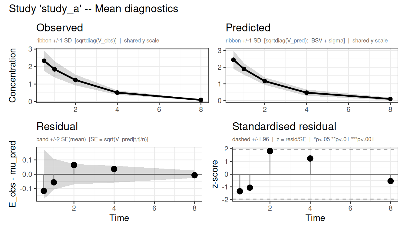
Figure 2: Observed vs predicted mean concentration (top) and residuals (bottom) for each study.
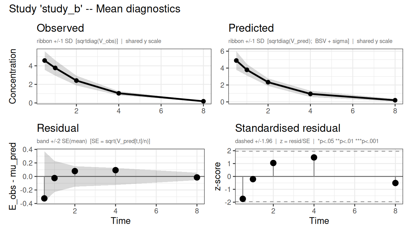
Figure 3: Observed vs predicted mean concentration (top) and residuals (bottom) for each study.
When only variances are available
When V is diagonal (as in the above example), admixr2 automatically sets method = "var" and uses only the marginal variances in the likelihood. If you have the full covariance matrix - for example if the original authors shared it, or if you derived it from a published model - pass a full symmetric matrix and admixr2 will use method = "cov" automatically.
Usecase 2: published NLME models as data source
Sometimes you do not have the (digitized) PK summary, but you do have published pharmacometric models - papers or submissions with fixed-effect estimates, IIV, and residual error. Each published model implicitly defines a probability distribution over concentration-time profiles; datagen() makes that distribution explicit by sampling it and computing the population mean and full covariance matrix.
A key advantage of using the model as a starting point over (digitized) summary data: the full V matrix can be estimated, which also captures the within-subject correlation across time points. A variance-only summary discards this structure; a published model can be used to recover it.
In practice, different publications often used different structural models for the same compound, usually because they sampled differently. admixr2 can be used to make a model based on models with different structures as well.
Here we present an example with two toy studies: the first study sampled at steady state, taking only a peak and a trough each interval - a sparse design that characterises exposure but never shows the shape of the decline, so a one-compartment model was all it could support. The second study was a richly sampled single-dose study that followed the concentration well into the terminal tail, and that long tail exposed a clear distribution phase, which was fit using a two-compartment model. The original authors’ choices are fixed - but you can choose any model as analysis model. datagen() supports per-study model elements so that the simulated aggregate data reflects the study design of the published model.
# Study 1 sampled at steady state, peak and trough only; study 2 followed a
# single dose out to the long terminal tail
times_1 <- c(1.5, 8)
times_2 <- c(0.5, 1, 2, 4, 8, 12, 24, 48)

# Study 1: 1-cmt oral model, 150 mg q8h, n = 80 (steady-state peak/trough)
model_study1 <- function() {
  ini({
    tcl     <- log(15)
    tv      <- log(58)
    tka     <- log(1.2)
    prop.sd <- c(0, 0.20)
    eta.cl  ~ 0.09
    eta.v   ~ 0.04
    eta.ka  ~ 0.04
  })
  model({
    cl <- exp(tcl + eta.cl)
    v  <- exp(tv  + eta.v)
    ka <- exp(tka + eta.ka)
    d/dt(depot)   <- -ka * depot
    d/dt(central) <-  ka * depot - (cl / v) * central
    cp <- central / v
    cp ~ prop(prop.sd)
  })
}

# Study 2: 2-cmt oral model, 300 mg, n = 200 (long terminal sampling)
model_study2 <- function() {
  ini({
    tcl     <- log(14)
    tv1     <- log(40)
    tv2     <- log(25)
    tq      <- log(8)
    tka     <- log(1.0)
    prop.sd <- c(0, 0.18)
    eta.cl  ~ 0.09
    eta.v1  ~ 0.04
    eta.ka  ~ 0.04
  })
  model({
    cl <- exp(tcl + eta.cl)
    v1 <- exp(tv1 + eta.v1)
    v2 <- exp(tv2)
    q  <- exp(tq)
    ka <- exp(tka + eta.ka)
    d/dt(depot)      <- -ka * depot
    d/dt(central)    <-  ka * depot - (cl + q) / v1 * central + q / v2 * peripheral
    d/dt(peripheral) <-  q / v1 * central - q / v2 * peripheral
    cp <- central / v1
    cp ~ prop(prop.sd)
  })
}
Each study carries its own model element, and datagen() simulates that study from it.
published_data <- datagen(
  studies = list(
    study1 = list(
      model = model_study1,
      times = times_1,
      ev    = et(amt = 150, ii = 8, ss = 1),
      n     = 80L
    ),
    study2 = list(
      model = model_study2,
      times = times_2,
      ev    = et(amt = 300),
      n     = 200L
    )
  ),
  control = datagenControl(n_sim = 10000L)
)
Now fit your own analysis model jointly to both studies. Your model does not need to match either published structure - here we use a one-compartment model to find the CL and V that best reconcile both datasets:
analysis_oral <- function() {
  ini({
    tcl     <- log(12)
    tv      <- log(50)
    tka     <- log(1.5)
    prop.sd <- c(0, 0.25)
    eta.cl  ~ 0.12
    eta.v   ~ 0.06
    eta.ka  ~ 0.06
  })
  model({
    cl <- exp(tcl + eta.cl)
    v  <- exp(tv  + eta.v)
    ka <- exp(tka + eta.ka)
    d/dt(depot)   <- -ka * depot
    d/dt(central) <-  ka * depot - (cl / v) * central
    cp <- central / v
    cp ~ prop(prop.sd)
  })
}
fit_mbma <- nlmixr2(
analysis_oral, admData(), est = "admc",
control = admControl(
studies = published_data, # study1 and study2
n_sim = 2000L,
covMethod = "r",
cores = 10
)
)The aggregate likelihood sums across both studies, each weighted by its own sample size \(n\), so study 2 (n = 200) contributes more than study 1 (n = 80).
A one-compartment analysis model cannot perfectly reproduce a two-compartment covariance, so the result is a compromise between the two parameterisations rather than an exact reconciliation; the full V from study 2 still contributes, because its between-time correlation enters the likelihood rather than being discarded.
Combining both approaches
A combination of observed and model-derived data can be estimated in a single model fit. Both produce the same needed inputs (E, V, n), so the estimator treats them identically:
# IV digitized studies + oral MBMA studies in one call
# (requires a model that handles both routes; simplified here for illustration)
all_studies <- c(
  list(study_a = study_a, study_b = study_b),
  published_data   # adds study1 and study2
)

fit_joint <- nlmixr2(
  analysis_oral, admData(), est = "admc",
  control = admControl(
    studies   = all_studies,
    n_sim     = 2000L,
    covMethod = "r",
    cores = 10
  )
)
This is where aggregate data modelling becomes most powerful: the full published literature - digitized IV profiles, model-derived oral studies, competitor models - all contribute to a single model with parameter estimates, and you get proper uncertainty quantification from the combined likelihood.
Getting started
admixr2 is on CRAN:
install.packages("admixr2")but we recommend to install the stable development version from GitHub, currently v0.2.0, which includes the latest features and bug fixes:
pak::pak("LeidenPharmacology/admixr2@v0.2.0")The package documentation at https://leidenpharmacology.github.io/admixr2 includes vignettes on all four estimators, the datagen() workflow, multi-study fitting, and diagnostic plots. The mathematical foundations - the aggregate likelihood, the CRN analytical gradient, and the IRMC algorithm - are described in detail in the Mathematics of aggregate data modelling article.
Acknowledgements
admixr2 builds on the aggregate data likelihood first described by Välitalo et al. (2021) and implemented in admr by van de Beek et al. (2025). We want to thank the nlmixr2 development team for the rxode2 and nlmixr2est infrastructure that admixr2 is built on.
- Posted on:
- July 2, 2026
- Length:
- 10 minute read, 2114 words
- Categories:
- nlmixr2
- Tags:
- meta-analysis MBMA aggregate-data
- See Also: