nlmixr2 Neural Network ODEs with pmxNODE
By Matthew Fidler in nlmixr2 pmxNODE
April 30, 2025
Neural Network ODEs and nlmixr2
I have had some requests to talk about nlmixr2 using neural network
ODEs, since neural networks are something that more people are
exploring with the explosion of artificial intelligence LLMs.
There is a package, pmxNODE, by Dominic Bräm that adds neural network
ODEs to pharmacometric modeling tools like NONMEM, Monolix and
nlmixr2.
In addition to the code that Dominic has added, I extended this
package to allow Neural Networks directly in a rxode2 or nlmixr2
model. I will go through an annotated example to show how these can
be used directly in the nlmixr2 model. Currently the pmxNODE does
not have any nlmixr2 examples in their inst directory, so I will
adapt their NONMEM example to use in nlmixr2:
library(nlmixr2)
library(pmxNODE)

d <- read.csv(system.file("data_example1_nm.csv", package="pmxNODE"),
              na.strings=".")

ex1 <- function()  {
  ini({
    lV <- 2
    add.sd <- .1
    prop.sd <- .1
  })
  model({
    V <- lV
    d/dt(central) <- NN(c, state=central, min_init=0.5, max_init=5) +
      DOSE * NN(t, state=t, min_init=1, max_init=5, time_nn=TRUE)
    Cc <- central/V
    Cc ~ prop(prop.sd) + add(add.sd)
  })
}
This example has 2 neural networks, one related to the central state
(labeled c) with a minimum activation point of 0.5 and maximum
activation point of 5. The second is a time-based neural network that
moderates the dose. This has a minimum activation point of 1 and a
maximum activation of 5 (and is called out as a time neural network by
time_nn=TRUE, and labeled with t). While these neural networks
may take care of both elimination and absorption independently (with
elimination in the central neural network and dosing in the
time-neural network), they may not be completely independent since
they are neural networks.
In general, the NN function is implemented by the rxode2 language
extension described
here,
but done in the pmxNODE package. This means that the NN()
function will only be available if you load the pmxNODE package.
The NN() function has the form:
Neural Network identifier, required can be a name or a number;
state=defines the state to be used in theNN(). For time, uset.min_init=defines the minimal activation point for theNN(), i.e., minimal expected state.max_init=defines the maximal activation point for theNN(), i.e., maximal expected state.n_hidden=(optional) defines the number of neurons in the hidden layer, default is5.act=(optional) defines activation function in the hidden layer,ReLUandSoftplusimplemented, default isReLU().time_nn=(optional) defines whether theNN()should be assumed to be a time-dependentNN()and consequently all weights from input to hidden layer should be strictly negative.
For more information about how to use these functions, I suggest
reading the articles related to pmxNODE:
Since this extra neural network function is a special user function in
the pmxNODE, not only does it mean that you need to load the package
to use it with nlmixr2, it also means that the full function is
evaluated when evaluating the UI:
m1 <- ex1()
m2 <- ex1()
# You can see the full code by printing the function:
print(m1)
## ── rxode2-based free-form 1-cmt ODE model ──────────────────────────────────────────────────────
## ── Initalization: ──
## Fixed Effects ($theta):
##      lV  add.sd prop.sd  lWc_11  lWc_12  lWc_13  lWc_14  lWc_15  lbc_11  lbc_12
##   2.000   0.100   0.100   0.100   0.100   0.200  -0.100   0.100  -0.145  -0.482
##  lbc_13  lbc_14  lbc_15  lWc_21  lWc_22  lWc_23  lWc_24  lWc_25  lbc_21  lWt_11
##  -0.646   0.464  -0.292  -0.100   0.100   0.100   0.100  -0.200   0.100   0.100
##  lWt_12  lWt_13  lWt_14  lWt_15  lbt_11  lbt_12  lbt_13  lbt_14  lbt_15  lWt_21
##  -0.200  -0.100  -0.100   0.200   0.026   0.143   0.038   0.016   0.195   0.200
##  lWt_22  lWt_23  lWt_24  lWt_25
##   0.100  -0.300   0.300  -0.100
##
## States ($state or $stateDf):
## Compartment Number Compartment Name
## 1 1 central
## ── Model (Normalized Syntax): ──
## function() {
## ini({
## lV <- 2
## add.sd <- c(0, 0.1)
## prop.sd <- c(0, 0.1)
## lWc_11 <- 0.1
## lWc_12 <- 0.1
## lWc_13 <- 0.2
## lWc_14 <- -0.1
## lWc_15 <- 0.1
## lbc_11 <- -0.145
## lbc_12 <- -0.482
## lbc_13 <- -0.646
## lbc_14 <- 0.464
## lbc_15 <- -0.292
## lWc_21 <- -0.1
## lWc_22 <- 0.1
## lWc_23 <- 0.1
## lWc_24 <- 0.1
## lWc_25 <- -0.2
## lbc_21 <- 0.1
## lWt_11 <- 0.1
## lWt_12 <- -0.2
## lWt_13 <- -0.1
## lWt_14 <- -0.1
## lWt_15 <- 0.2
## lbt_11 <- 0.026
## lbt_12 <- 0.143
## lbt_13 <- 0.038
## lbt_14 <- 0.016
## lbt_15 <- 0.195
## lWt_21 <- 0.2
## lWt_22 <- 0.1
## lWt_23 <- -0.3
## lWt_24 <- 0.3
## lWt_25 <- -0.1
## })
## model({
## V <- lV
## Wc_11 <- lWc_11
## Wc_12 <- lWc_12
## Wc_13 <- lWc_13
## Wc_14 <- lWc_14
## Wc_15 <- lWc_15
## bc_11 <- lbc_11
## bc_12 <- lbc_12
## bc_13 <- lbc_13
## bc_14 <- lbc_14
## bc_15 <- lbc_15
## Wc_21 <- lWc_21
## Wc_22 <- lWc_22
## Wc_23 <- lWc_23
## Wc_24 <- lWc_24
## Wc_25 <- lWc_25
## bc_21 <- lbc_21
## hc_1 = Wc_11 * central + bc_11
## hc_2 = Wc_12 * central + bc_12
## hc_3 = Wc_13 * central + bc_13
## hc_4 = Wc_14 * central + bc_14
## hc_5 = Wc_15 * central + bc_15
## if (hc_1 < 0) {
## hc_1 <- 0
## }
## if (hc_2 < 0) {
## hc_2 <- 0
## }
## if (hc_3 < 0) {
## hc_3 <- 0
## }
## if (hc_4 < 0) {
## hc_4 <- 0
## }
## if (hc_5 < 0) {
## hc_5 <- 0
## }
## NNc = Wc_21 * hc_1 + Wc_22 * hc_2 + Wc_23 * hc_3 + Wc_24 *
## hc_4 + Wc_25 * hc_5 + bc_21
## Wt_11 <- lWt_11
## Wt_12 <- lWt_12
## Wt_13 <- lWt_13
## Wt_14 <- lWt_14
## Wt_15 <- lWt_15
## bt_11 <- lbt_11
## bt_12 <- lbt_12
## bt_13 <- lbt_13
## bt_14 <- lbt_14
## bt_15 <- lbt_15
## Wt_21 <- lWt_21
## Wt_22 <- lWt_22
## Wt_23 <- lWt_23
## Wt_24 <- lWt_24
## Wt_25 <- lWt_25
## ht_1 = -Wt_11^2 * t + bt_11
## ht_2 = -Wt_12^2 * t + bt_12
## ht_3 = -Wt_13^2 * t + bt_13
## ht_4 = -Wt_14^2 * t + bt_14
## ht_5 = -Wt_15^2 * t + bt_15
## if (ht_1 < 0) {
## ht_1 <- 0
## }
## if (ht_2 < 0) {
## ht_2 <- 0
## }
## if (ht_3 < 0) {
## ht_3 <- 0
## }
## if (ht_4 < 0) {
## ht_4 <- 0
## }
## if (ht_5 < 0) {
## ht_5 <- 0
## }
## NNt = Wt_21 * ht_1 + Wt_22 * ht_2 + Wt_23 * ht_3 + Wt_24 *
## ht_4 + Wt_25 * ht_5
## d/dt(central) <- NNc + DOSE * NNt
## Cc <- central/V
## Cc ~ prop(prop.sd) + add(add.sd)
## })
## }Note that the initial estimates are chosen at random for the neural
network ODE function, you can see that the initial estimates of the
functions m1 and m2:
m1$theta## lV add.sd prop.sd lWc_11 lWc_12 lWc_13 lWc_14 lWc_15 lbc_11 lbc_12
## 2.000 0.100 0.100 0.100 0.100 0.200 -0.100 0.100 -0.145 -0.482
## lbc_13 lbc_14 lbc_15 lWc_21 lWc_22 lWc_23 lWc_24 lWc_25 lbc_21 lWt_11
## -0.646 0.464 -0.292 -0.100 0.100 0.100 0.100 -0.200 0.100 0.100
## lWt_12 lWt_13 lWt_14 lWt_15 lbt_11 lbt_12 lbt_13 lbt_14 lbt_15 lWt_21
## -0.200 -0.100 -0.100 0.200 0.026 0.143 0.038 0.016 0.195 0.200
## lWt_22 lWt_23 lWt_24 lWt_25
## 0.100 -0.300 0.300 -0.100m2$theta## lV add.sd prop.sd lWc_11 lWc_12 lWc_13 lWc_14 lWc_15 lbc_11 lbc_12
## 2.000 0.100 0.100 0.100 -0.100 -0.200 -0.200 0.100 -0.381 0.153
## lbc_13 lbc_14 lbc_15 lWc_21 lWc_22 lWc_23 lWc_24 lWc_25 lbc_21 lWt_11
## 0.881 0.129 -0.279 0.200 0.300 -0.200 0.100 -0.200 0.200 0.200
## lWt_12 lWt_13 lWt_14 lWt_15 lbt_11 lbt_12 lbt_13 lbt_14 lbt_15 lWt_21
## -0.200 0.200 0.200 -0.200 0.158 0.138 0.097 0.115 0.103 0.200
## lWt_22 lWt_23 lWt_24 lWt_25
## 0.200 -0.200 -0.200 -0.300To make sure your analyses are reproducible with the Neural Network models, you need to then set the seed.
set.seed(42)
ex1 <- ex1()
It may be more helpful to have a population-only model with a neural network and then add between subject variability to the model.
fit <- suppressMessages(nlmixr(ex1, d, "bobyqa", control=list(print=0)))## |-----+---------------+-----------+-----------+-----------+-----------|p <- plot(fit)
# Here I am subsetting the plots to show only individual plots
p <- p[["All Data"]]
# In this case the list of plots is named starting with "individual"
w <- which(vapply(names(p), function(x) grepl("individual", x), logical(1)))
# This creates a new list of plots, and changes it to the same class
# as output by nlmixr2
p <- lapply(w,function(x) p[[x]])
class(p) <- "nlmixr2PlotList"
p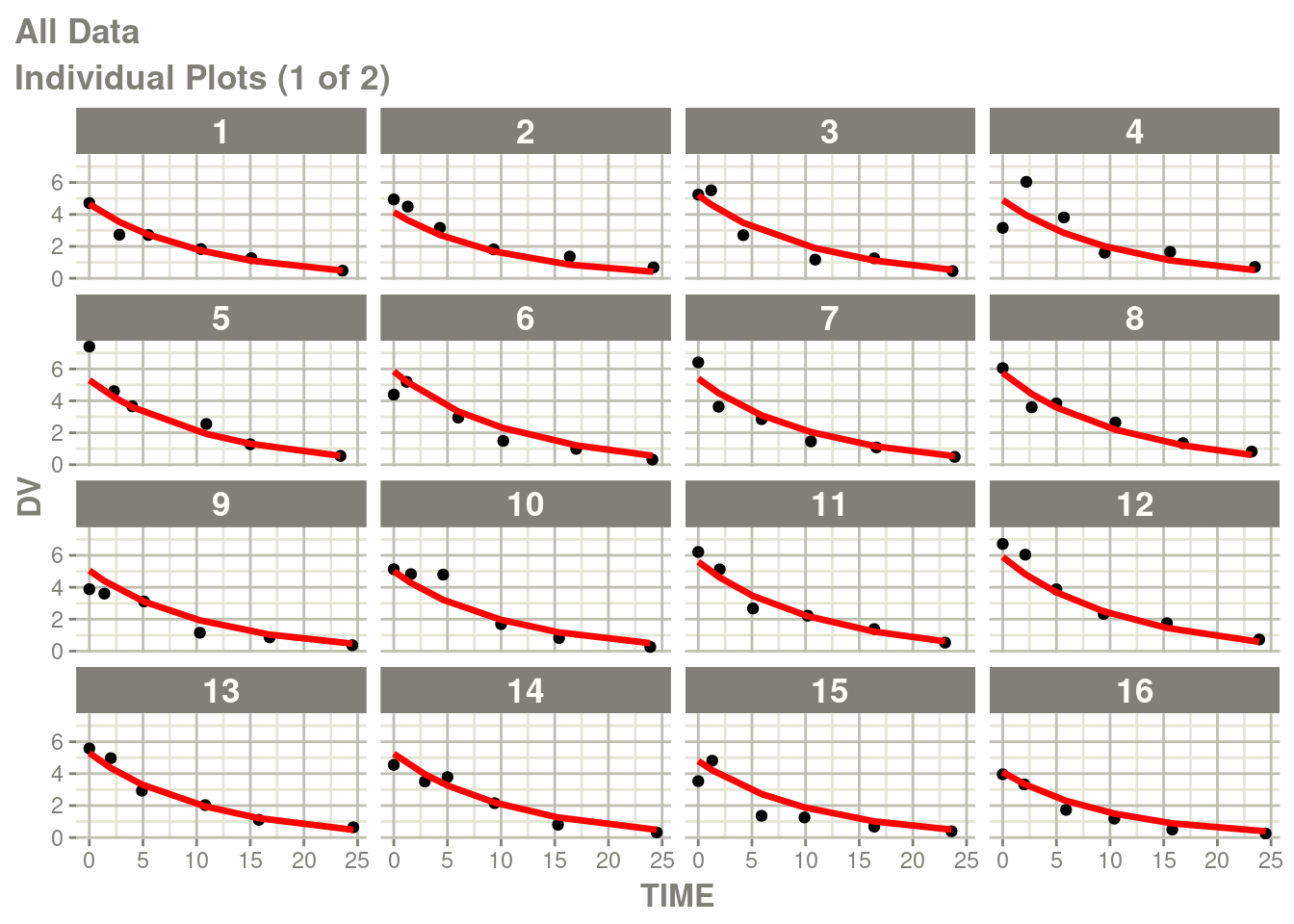
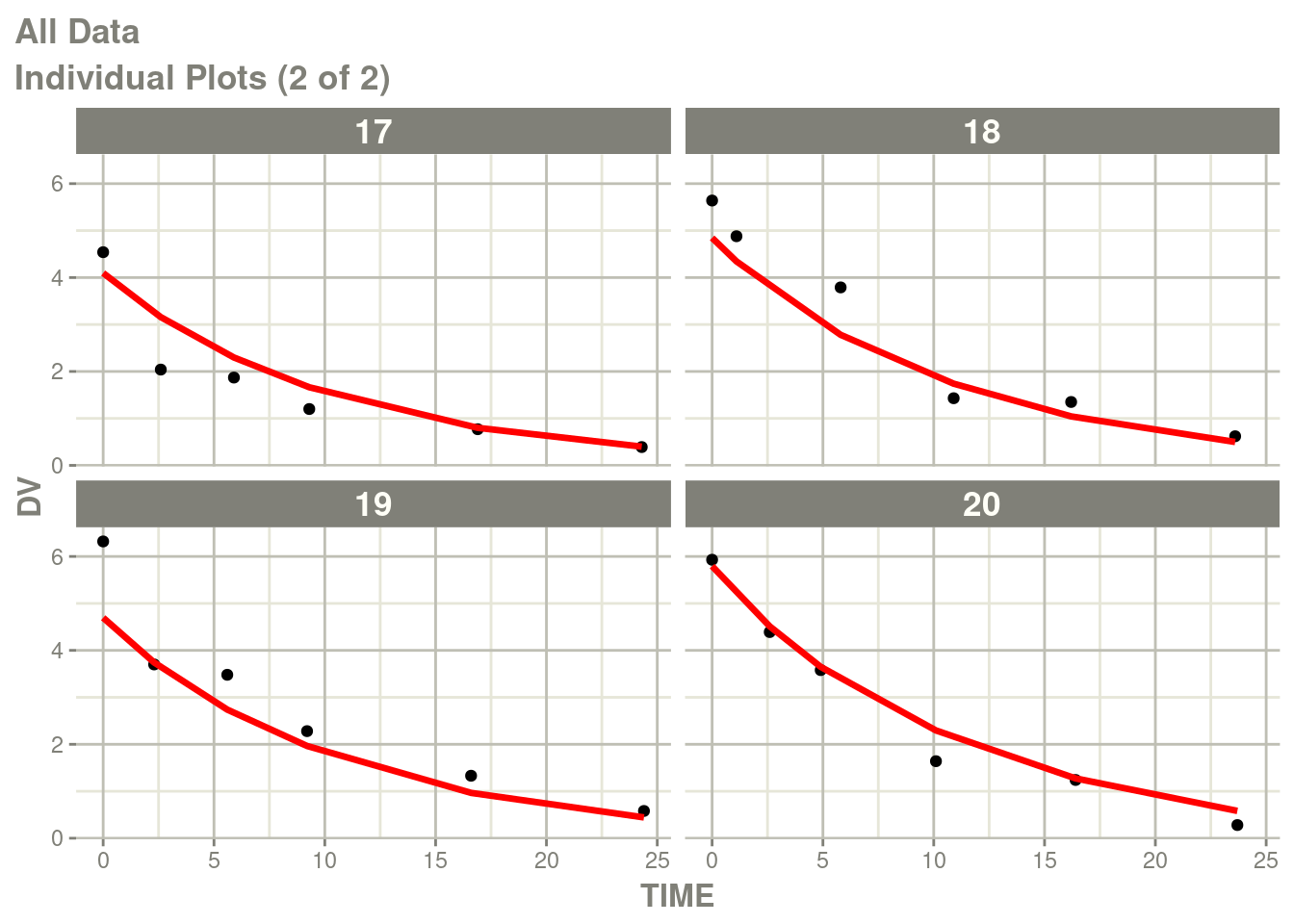
You can see there is no between subject variability on the Neural
Network, you can add it (with the best estimates) with the function
NNbsv(). Note this function is not yet part of the pmxNODE
package, details are below.
newModel <- fit %>%
  model(V <- lV*exp(eta.V)) %>%
  ini(eta.V ~ .1) %>%
  NNbsv()
## ℹ add between subject variability `eta.V` and set estimate to 1## ℹ change initial estimate of `eta.V` to `0.1`fit2 <- suppressMessages(nlmixr2(newModel, d, "focei", control=foceiControl(print=0)))## calculating covariance matrix
## doneNote the NNbsv() is a recent addition to pmxNODE and needs to be
reviewed to added to the package. The pull request adds this
function to the package.
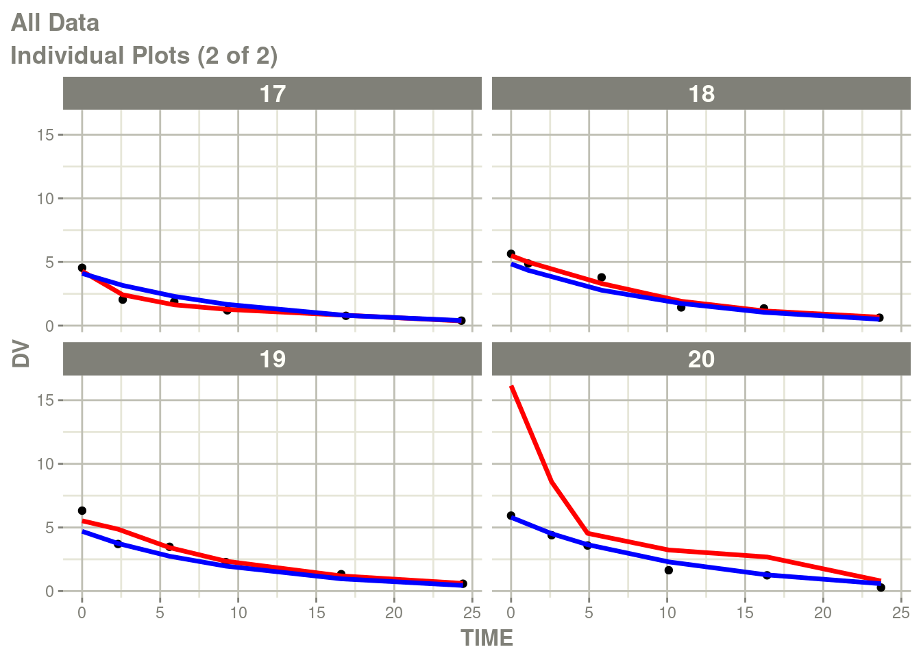
You can see the differences here:
p <- plot(fit2)

# Here I am subsetting the plots to show only individual plots
p <- p[["All Data"]]

# In this case the list of plots is named starting with "individual"
w <- which(vapply(names(p), function(x) grepl("individual", x), logical(1)))

# This creates a new list of plots, and changes it to the same class
# as output by nlmixr2
p <- lapply(w, function(x) p[[x]])
class(p) <- "nlmixr2PlotList"

p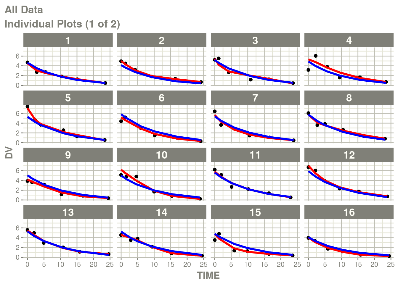
Other activation and NN functions in rxode2/nlmixr2 in the future.
rxode2 has implemented many neural-network activation functions
built-in. In the future packages like pmxNODE may use these
directly and even extend to use some of the other neural network
functions there. Since they are built-into rxode2, the models may be
a bit faster if this integration occurs.
NNbsv() function
Since the pull request hasn’t been accepted at this point, I am providing the code below in case you want to use it yourself:
NNbsv <- function(ui, val=0.1, str="%s <- l%s*exp(eta.%s)") {
  .ui <- rxode2::assertRxUi(ui)
  .n <- names(.ui$theta)
  .etaNames <- dimnames(.ui$omega)[[1]]
  .nn <- vapply(seq_along(.n), function(i){
    grepl("^[l][Wb].*_[1-9]?[0-9]*", .n[i]) &&
      !any(paste0("eta.", .n[i]) %in% .etaNames)
  }, logical(1))
  .n <- .n[which(.nn)]
  if (length(.n) == 0) return(ui)
  .v <- gsub("^[l]", "", .n)
  .s1 <- paste0(.v, " <- l", .v)
  .s2 <- sprintf(str, .v, .v, .v)
  # Change the model expression first.
  .model <- vapply(.ui$lstChr,
                   function(l) {
                     .w <- which(.s1 == l)
                     if (length(.w) != 1) {
                       return(l)
                     }
                     .s2[.w]
                   }, character(1),
                   USE.NAMES=FALSE)
  rxode2::model(.ui) <- .model
  # Now add eta estimates
  .iniDf <- .ui$iniDf
  .w <- which(!is.na(.iniDf$neta1))
  if (length(.w) == 0L) {
    .maxEta <- 0
  } else {
    .maxEta <- max(.iniDf$neta1[.w])
  }
  .i1 <- .iniDf[1,]
  .i1$ntheta <- NA_integer_
  .i1$lower <- -Inf
  .i1$upper <- Inf
  .i1$est <- val
  .i1$label <- NA_character_
  .i1$backTransform <- NA_character_
  .i1$condition <- "id"
  .i1$err <- NA_character_
  .etas <- do.call(`rbind`,
                   lapply(seq_along(.v), function(i) {
                     .cur <- .i1
                     .cur$neta1 <- .maxEta+i
                     .cur$neta2 <- .maxEta+i
                     .cur$name <- paste0("eta.", .v[i])
                     .cur
                   }))
  .iniDf <- rbind(.iniDf, .etas)

  rxode2::ini(.ui) <- .iniDf
  .ui
}