nlmixr2/rxode2 exploring data with rxode2 geoms

geom_amt() – exploring when dosing occurs

rxode2 will allow exploring time of dosing with the geom_amt(). From the geom_amt() documentation we can see how this is applied:

library(rxode2)
library(units)

## udunits database from /usr/share/xml/udunits/udunits2.xml

library(ggplot2)

mod1 <- function() {
  ini({
    KA <- 2.94E-01
    CL <- 1.86E+01
    V2 <- 4.02E+01
    Q  <- 1.05E+01
    V3 <- 2.97E+02
    Kin <- 1
    Kout <- 1
    EC50 <- 200
  })
  model({
    C2 <- centr/V2
    C3 <- peri/V3
    d/dt(depot) <- -KA*depot
    d/dt(centr) <-  KA*depot - CL*C2 - Q*C2 + Q*C3
    d/dt(peri)  <-                    Q*C2 - Q*C3
    d/dt(eff)   <- Kin - Kout*(1-C2/(EC50+C2))*eff
  })
}

## These are making the more complex regimens of the rxode2 tutorial

## bid for 5 days
bid <- et(timeUnits="hr") %>%
  et(amt=10000,ii=12,until=set_units(5, "days"))

## qd for 5 days
qd <- et(timeUnits="hr") %>%
  et(amt=20000,ii=24,until=set_units(5, "days"))

## bid for 5 days followed by qd for 5 days

et <- seq(bid,qd) %>% et(seq(0,11*24,length.out=100))

bidQd <- rxSolve(mod1, et, addDosing=TRUE)

## ℹ parameter labels from comments are typically ignored in non-interactive mode

## ℹ Need to run with the source intact to parse comments

## using C compiler: ‘gcc (Ubuntu 11.4.0-1ubuntu1~22.04) 11.4.0’

# by default dotted and under-stated
plot(bidQd, C2) + geom_amt(aes(amt=amt))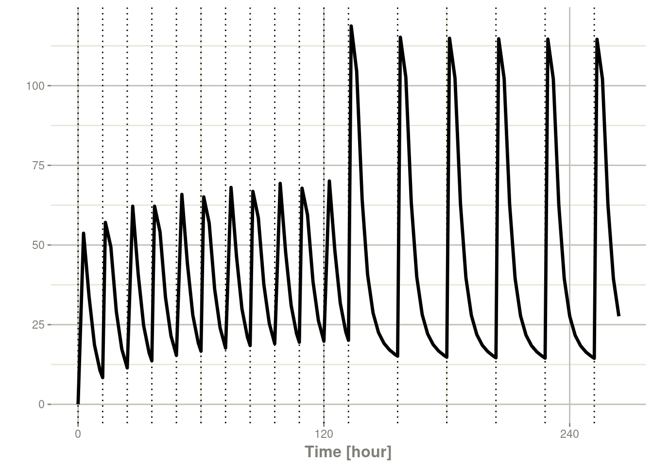

# of course you can make it a bit more visible

plot(bidQd, C2) + geom_amt(aes(amt=amt), col="red", lty=1, linewidth=1.2)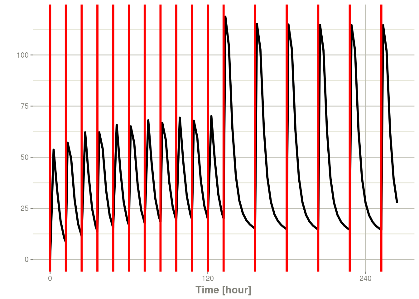

While not terribly complicated it is a convenient way to add dosing to your ggplot2 object.

geom_cens() – exploring what the censoring means

Another useful way to see how your data is censored (according to nlmixr2 and Monolix) is to use the geom_cens() function:

library(rxode2)
library(ggplot2)
library(tidyverse)

## ── Attaching core tidyverse packages ──────────────────────────────────────── tidyverse 2.0.0 ──
## ✔ dplyr     1.1.4     ✔ readr     2.1.5
## ✔ forcats   1.0.0     ✔ stringr   1.5.1
## ✔ lubridate 1.9.4     ✔ tibble    3.2.1
## ✔ purrr     1.0.4     ✔ tidyr     1.3.1
## ── Conflicts ────────────────────────────────────────────────────────── tidyverse_conflicts() ──
## ✖ dplyr::filter() masks stats::filter()
## ✖ dplyr::lag()    masks stats::lag()
## ℹ Use the conflicted package (<http://conflicted.r-lib.org/>) to force all conflicts to become errors

library(xgxr)

# Get the data from xgxr
pkpd_data <-
  case1_pkpd %>%
  arrange(DOSE) %>%
  select(-IPRED) %>%
  mutate(TRTACT_low2high = factor(TRTACT, levels = unique(TRTACT)),
         TRTACT_high2low = factor(TRTACT, levels = rev(unique(TRTACT))),
         DAY_label = paste("Day", PROFDAY),
         DAY_label = ifelse(DAY_label == "Day 0","Baseline",DAY_label))

pk_data <- pkpd_data %>%
  filter(CMT == 2)

pk_data_cycle1 <- pk_data %>%
  filter(CYCLE == 1)


ggplot(data = pk_data_cycle1, aes(x = TIME, y = LIDV)) +
  geom_line(aes(group = ID), color = "grey50", linewidth = 1, alpha = 0.3) +
  geom_cens(aes(cens=CENS)) +
  xgx_geom_ci(aes(x = NOMTIME, color = NULL, group = NULL, shape = NULL), conf_level = 0.95) +
  xgx_scale_y_log10() +
  xgx_scale_x_time_units(units_dataset = "hours", units_plot = "days") +
  labs(y = "Concentration (ng/ml)", color = "Dose") +
  theme(legend.position = "none") +
  facet_grid(.~TRTACT_low2high)

## Warning in geom_cens(aes(cens = CENS)): Ignoring unknown aesthetics: cens

## Warning: Using the `size` aesthetic in this geom was deprecated in ggplot2 3.4.0.
## ℹ Please use `linewidth` in the `default_aes` field and elsewhere instead.
## This warning is displayed once every 8 hours.
## Call `lifecycle::last_lifecycle_warnings()` to see where this warning was generated.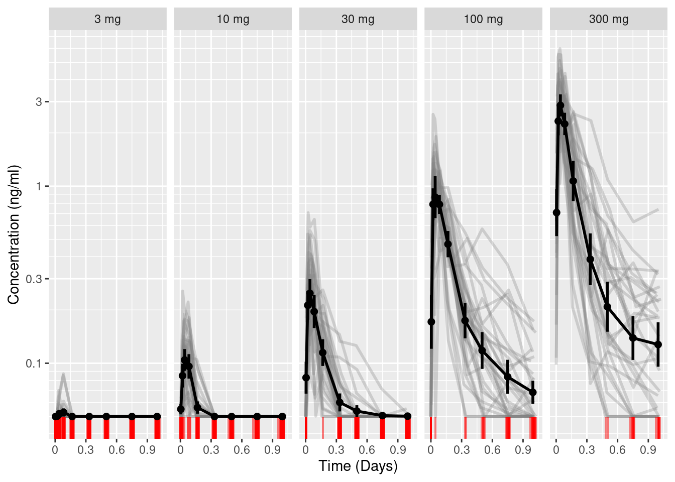

Whenever a point is censored, it shows the censoring assumptions by drawing a small box where the censoring occurs.

This is adapted from the nlmixr2 xgxr and ggPMX vignette.