Dual absorption with one dose record

How this is usually done

In NONMEM, the usual approach is to put the dose in the data twice: one record with CMT=1 and an identical one with CMT=2. The model then sets F1 = FR and F2 = 1 - FR so each copy carries its share. This works, but the dataset no longer describes what was given and requires you to rewrite the dataset every time you want to try a new absorption model. (This is true about compartment numbers too, this is why nlmixr2 and rxode2 can use named compartments)

Monolix avoids the duplication with its PK macros: you write two absorption() macros against the same adm and give each a share p (and, if needed, its own Tlag or Tk0). The data keeps one row per dose, and the model decides where the dose goes.

rxode2 and nlmixr2 now work the same way. A splitting directive in the model({}) block tells rxode2 to take each dose recorded against one compartment and send a copy to each of several others. The dataset keeps one row per dose, exactly as it was given. Since nlmixr2 estimates with rxode2 models, the same directive works when you fit.

Everything below works with the current CRAN releases (rxode2 5.1.8 and nlmixr2est 7.2.1).

The four directives

directive	bolus records become	infusion records become
splitBolus(src, a, b, ...)	a bolus in each target	left alone
splitInfusion(src, a, b, ...)	left alone	an infusion in each target
splitInfusionBolus(src, a, b, ...)	an infusion in a (the first target), a bolus in the others	an infusion in each target
splitBolusInfusion(src, a, b, ...)	a bolus in each target except the last, an infusion in the last	an infusion in each target

The same rules apply to all four:

• Every target receives the full amount. The directive copies the dose; it doesn’t divide it. Without any f(), each target gets the whole dose. To divide it, give each target a share with f(), for example f(depot) <- fr and f(slowdepot) <- 1 - fr. If you want the shares to add up to one, write them that way.

• Only one splitting directive is allowed per model.

• The source can be one of the targets. splitBolus(depot, depot, slowdepot) keeps part of the dose in depot and sends a copy to slowdepot. This is usually what you want: the data says depot, and depot is still one of the absorption routes. If you leave the source out of the target list, the dose doesn’t go there at all. The source is then only a label for the data, but it still needs an ODE (d/dt(sc) <- 0 is enough). The targets themselves must not repeat.

• You can split into as many compartments as you need. splitBolus(depot, depot, mid, slowdepot) gives the full amount to 3 compartments (depot, mid and slowdepot) and with an f() on each compartment you could share that amount in any way you want with that one dose record.

• One target moves the dose instead of splitting it. splitBolus(depot, slowdepot) sends every bolus recorded against depot to slowdepot, and depot gets nothing, even if it has its own ODE. splitInfusion(depot, slowdepot) does the same for infusions. This is useful when the data says CMT = depot but the model wants the dose somewhere else, such as the start of a transit chain. No f() is needed: the target gets the full dose.

• A dose type the directive doesn’t handle goes to the source unchanged. Under splitBolus(), an infusion recorded against depot goes into depot only and is not split. If the source isn’t a target (d/dt(sc) <- 0), it is never absorbed at all. If your data mixes boluses and infusions on the source, use one of the two mixed directives.

• alag(), f(), rate() and dur() on each target apply as usual. This means each route can have its own lag time.

Two first-order routes: splitBolus()

Here is the classic case: 60% of the dose absorbs quickly and 40% slowly. The dose stays in depot for the fast route, and a copy goes to slowdepot for the slow one:

dual <- function() {
  ini({
    tka1 <- log(1.5);  label("Fast absorption rate ka1 (1/h)")
    tka2 <- log(0.15); label("Slow absorption rate ka2 (1/h)")
    tfr  <- logit(0.6); label("Fraction absorbed by the fast route")
    tcl  <- log(4);    label("Clearance CL (L/h)")
    tv   <- log(40);   label("Volume V (L)")
    eta.ka1 ~ 0.1
    eta.cl  ~ 0.09
    eta.v   ~ 0.04
    prop.sd <- 0.1
  })
  model({
    ka1 <- exp(tka1 + eta.ka1)
    ka2 <- exp(tka2)
    fr  <- expit(tfr)
    cl  <- exp(tcl + eta.cl)
    v   <- exp(tv + eta.v)

    splitBolus(depot, depot, slowdepot) # one depot dose -> depot + slowdepot
    f(depot)     <- fr
    f(slowdepot) <- 1 - fr

    d/dt(depot)     <- -ka1 * depot       # fast route
    d/dt(slowdepot) <- -ka2 * slowdepot   # slow route
    d/dt(central)   <-  ka1 * depot + ka2 * slowdepot - cl / v * central
    cp <- central / v
    cp ~ prop(prop.sd)
  })
}

The event table has one dose, recorded against depot:

ev <- et(amt = 100, cmt = "depot") |> et(seq(0, 36, by = 0.25))

typical <- rxSolve(dual |> zeroRe(), ev)

typical |>
  as.data.frame() |>
  select(time, depot, slowdepot, central) |>
  pivot_longer(-time, names_to = "compartment", values_to = "amount") |>
  ggplot(aes(time, amount, color = compartment)) +
  geom_line(linewidth = 1) +
  labs(x = "Time (h)", y = "Amount (mg)",
       title = "One 100 mg dose, split 60/40 into a fast and a slow depot")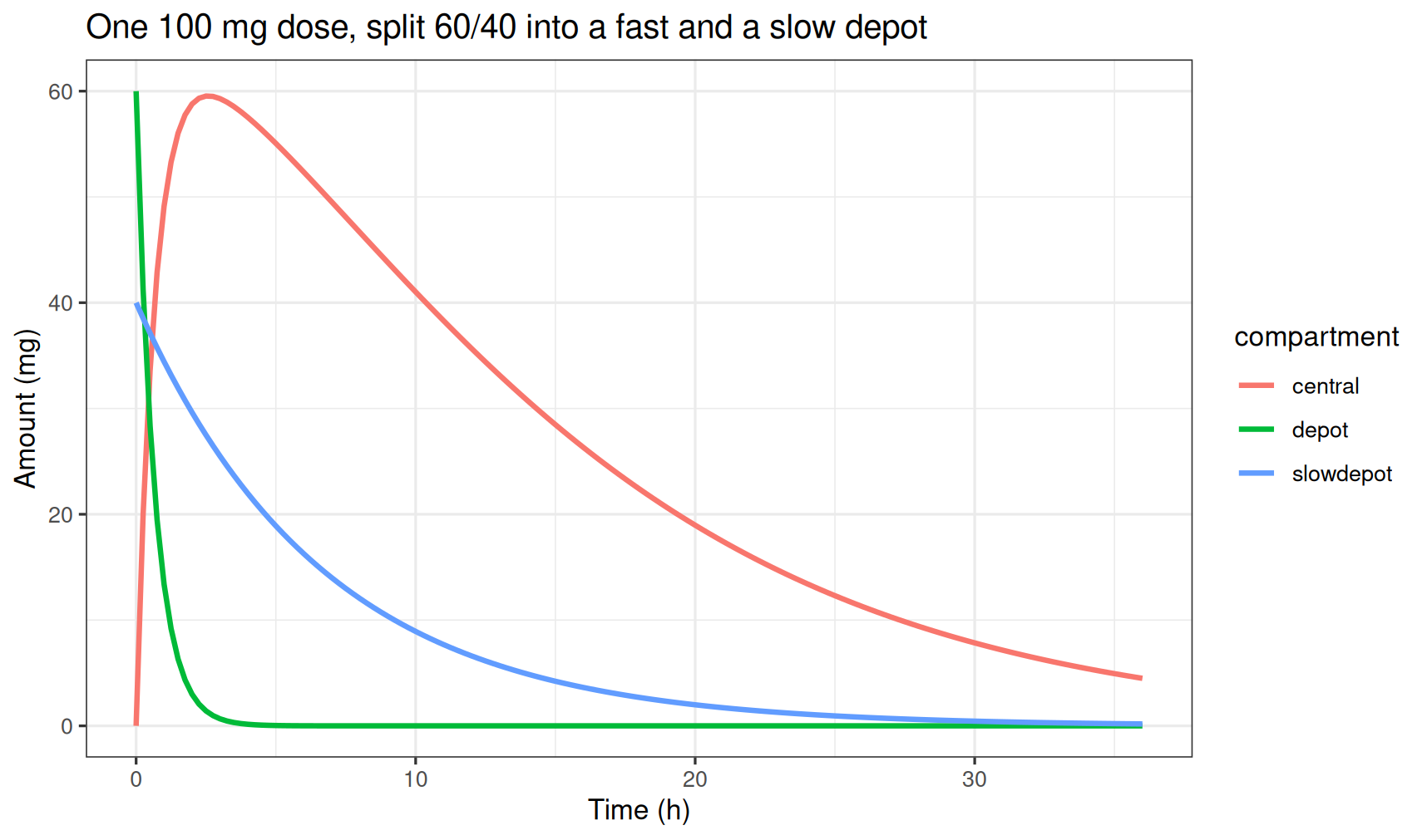

depot starts at 60 mg and empties within a few hours. slowdepot starts at 40 mg and is still emptying a day later.

To check the result, here is the NONMEM-style approach, with the dose entered twice and no directive. The two give the same answer:

twoRecords <- function() {
  ini({
    ka1 <- 1.5
    ka2 <- 0.15
    fr <- 0.6
    cl <- 4
    v <- 40
  })
  model({
    f(depot)     <- fr
    f(slowdepot) <- 1 - fr
    d/dt(depot)     <- -ka1 * depot
    d/dt(slowdepot) <- -ka2 * slowdepot
    d/dt(central)   <-  ka1 * depot + ka2 * slowdepot - cl / v * central
    cp <- central / v
  })
}
evTwice <- et(amt = 100, cmt = "depot") |>
  et(amt = 100, cmt = "slowdepot") |>
  et(seq(0, 36, by = 0.25))

all.equal(typical$cp, rxSolve(twoRecords, evTwice)$cp)

## [1] TRUE

Zero-order plus first-order: splitInfusionBolus()

Another common shape is a zero-order input straight into the central compartment (a constant release) combined with first-order absorption from the depot. The dose record is still a plain oral bolus. splitInfusionBolus() turns the bolus into a modeled infusion for the first target and a bolus for the others. The first target must declare dur() (or rate()) so rxode2 knows how long the infusion lasts:

zoFo <- function() {
  ini({
    tk0 <- 4;    label("Zero-order duration (h)")
    fr  <- 0.7;  label("Fraction by the zero-order route")
    ka2 <- 1.2;  label("First-order absorption rate (1/h)")
    lag2 <- 1.5; label("Lag time on the first-order route (h)")
    cl  <- 2
    v   <- 25
  })
  model({
    splitInfusionBolus(depot, central, depot)
    dur(central)  <- tk0          # central gets a 4 h zero-order input
    f(central)    <- fr
    f(depot)      <- 1 - fr
    alag(depot)   <- lag2         # the first-order part starts late

    d/dt(depot)   <- -ka2 * depot
    d/dt(central) <-  ka2 * depot - cl / v * central
    cp <- central / v
  })
}

zo <- rxSolve(zoFo, et(amt = 100, cmt = "depot") |> et(seq(0, 24, by = 0.1)))

ggplot(as.data.frame(zo), aes(time, cp)) +
  geom_line(linewidth = 1) +
  geom_vline(xintercept = c(1.5, 4), linetype = "dashed", color = "gray50") +
  labs(x = "Time (h)", y = "Concentration (mg/L)",
       title = "70% zero-order over 4 h, 30% first-order after a 1.5 h lag")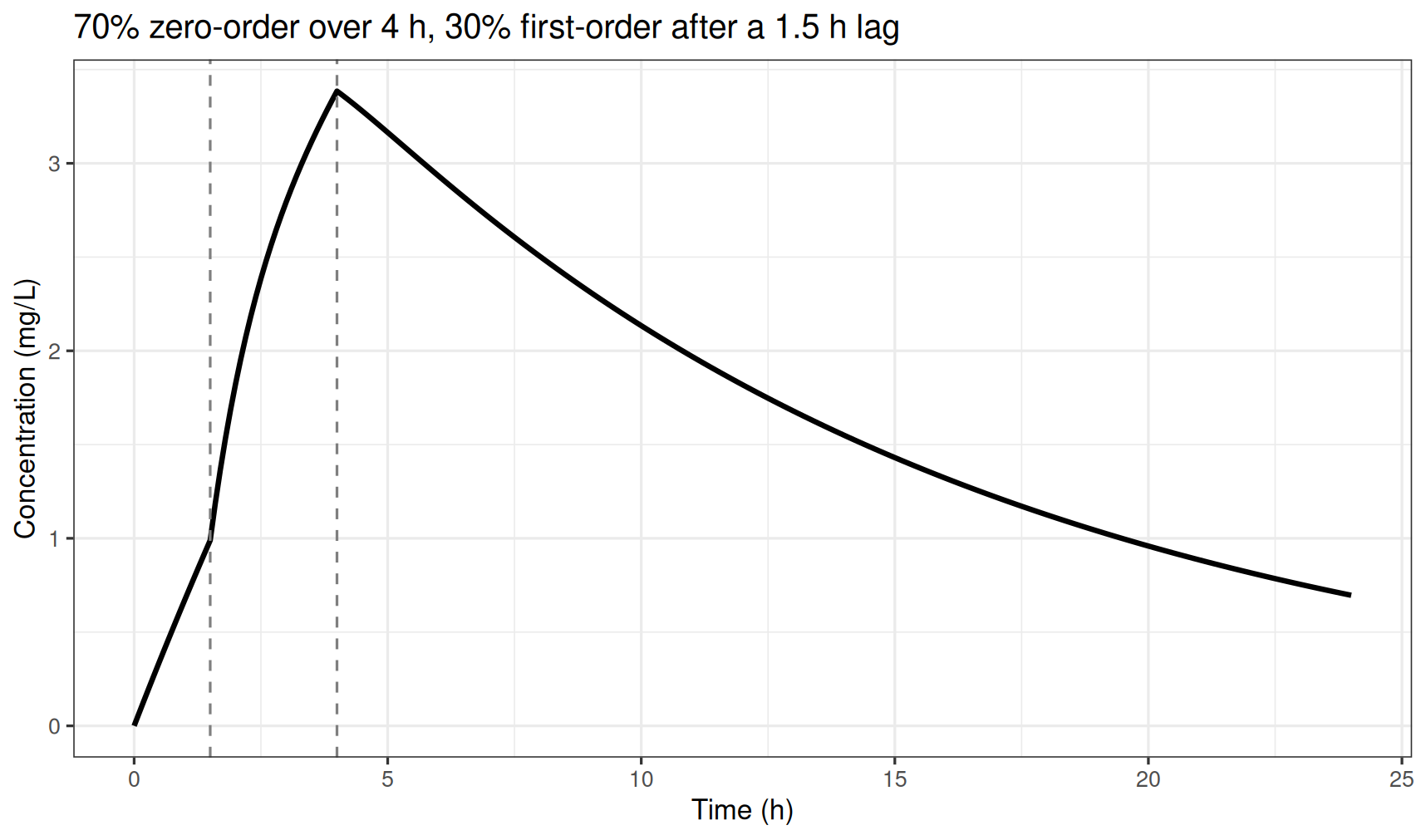

You can see the shape change at the lag time and again at the end of the zero-order input. splitBolusInfusion(depot, depot, central) describes the same model with the targets listed in the other order: there the last target receives the infusion. Use whichever reads better to you.

Both directives take any number of targets, but only one of them becomes an infusion, and its position is fixed: the first target for splitInfusionBolus(), the last for splitBolusInfusion(). Every other target gets a bolus. splitBolusInfusion(depot, depot, slowdepot, central) gives two first-order routes plus a zero-order input. A dur() on a target in the middle of the list is ignored, and that target silently gets a bolus.

Two details to watch. If the infusion target has no dur() or rate(), its copy silently stays a bolus, with no warning. And a steady-state bolus record (ss = 1) is not turned into an infusion: it is copied as a bolus to each target, and rxode2 warns you if the infusion target declared dur() or rate(). We will work to change this in the next release (you can track the issue here: (rxode2#1668))

Infusions in the data: splitInfusion()

splitInfusion() handles doses that are already infusions in the data, with a RATE or DUR column, or infusions from a modeled rate()/dur(). Each target gets its own copy of the infusion, and rxode2 moves the start and the stop records together so they still match. A subcutaneous infusion that drains through two pathways looks like this. This time the source, sc, is not a target: it is only the label in the data, so the whole infusion goes to fast and slow:

sc <- function() {
  ini({fr <- 0.6; ka1 <- 0.8; ka2 <- 0.05; cl <- 0.2; v <- 3})
  model({
    splitInfusion(sc, fast, slow)
    f(fast) <- fr
    f(slow) <- 1 - fr
    d/dt(sc)      <- 0
    d/dt(fast)    <- -ka1 * fast
    d/dt(slow)    <- -ka2 * slow
    d/dt(central) <-  ka1 * fast + ka2 * slow - cl / v * central
    cp <- central / v
  })
}

Remember that f() scales the amount. When you scale the amount of an infusion, rxode2 follows NONMEM: it holds fixed whichever of rate or duration the record gives.

If the record gives a rate, each copy keeps that rate and runs for a shorter time. If the record gives a dur, each copy keeps that duration and runs at a lower rate. The same 300 mg over 3 hours gives different profiles depending on how you write it:

byRate <- rxSolve(sc, et(amt = 300, rate = 100, cmt = "sc") |> et(seq(0, 24, by = 0.1)))
byDur  <- rxSolve(sc, et(amt = 300, dur = 3,    cmt = "sc") |> et(seq(0, 24, by = 0.1)))

bind_rows(
  as.data.frame(byRate) |> mutate(record = "rate = 100 mg/h (copies run 1.8 h and 1.2 h)"),
  as.data.frame(byDur)  |> mutate(record = "dur = 3 h (copies run at 60 and 40 mg/h)")
) |>
  ggplot(aes(time, cp, color = record)) +
  geom_line(linewidth = 1) +
  labs(x = "Time (h)", y = "Concentration (mg/L)", color = NULL) +
  theme(legend.position = "bottom")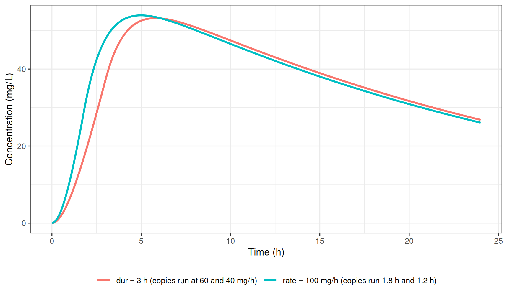

Neither is wrong, but you need to know which one your data means. For a physical infusion pump that ran for 3 hours, dur is probably what you want.

Estimation with nlmixr2

The directive is part of the model, so nlmixr2 uses it with every estimation method. The dataset stays the way the clinic recorded it: one dose row per dose, with CMT = depot.

First, simulate 60 subjects who each take 100 mg daily for three days, with a rich profile after the first and the last dose:

set.seed(2026)
rxSetSeed(2026)
nsub <- 60
sampleTimes <- c(0.25, 0.5, 1, 1.5, 2, 3, 4, 6, 8, 12, 16, 24,
                 48.5, 49, 50, 52, 54, 56, 60, 64, 72)

evPop <- et(amt = 100, cmt = "depot", ii = 24, addl = 2) |>
  et(sampleTimes) |>
  et(id = seq_len(nsub))

sim <- rxSolve(dual, evPop)

doses <- data.frame(ID = seq_len(nsub), TIME = 0, EVID = 1, AMT = 100,
                    II = 24, ADDL = 2, CMT = "depot", DV = NA)

obs <- as.data.frame(sim) |>
  transmute(ID = id, TIME = time, EVID = 0, AMT = 0, II = 0, ADDL = 0,
            CMT = "cp", DV = sim)

dat <- bind_rows(doses, obs) |> arrange(ID, TIME, desc(EVID))

head(dat, 4)

##   ID TIME EVID AMT II ADDL   CMT        DV
## 1  1 0.00    1 100 24    2 depot        NA
## 2  1 0.25    0   0  0    0    cp 0.5628164
## 3  1 0.50    0   0  0    0    cp 0.7948546
## 4  1 1.00    0   0  0    0    cp 1.1505977

Notice that the dataset never mentions slowdepot. The absorption model is in the model, and only there.

The example builds the dose rows directly rather than taking them from rxSolve(..., addDosing = TRUE). When a model splits its doses, the dose rows that addDosing returns are the translated records, one for depot and one for slowdepot. The output then has two dose rows per dose, which is the NONMEM-style data this approach is meant to avoid.

Now fit it with FOCEi and with SAEM. It’s the same model function and the same data:

fitF := nlmixr(dual, dat, "focei", control = foceiControl(print = 0))
fitS := nlmixr(dual, dat, "saem",  control = saemControl(print = 0))

truth <- c(tka1 = 1.5, tka2 = 0.15, tfr = 0.6, tcl = 4, tv = 40)

est <- function(fit, method) {
  fit$parFixedDf[names(truth), ] |>
    mutate(parameter = names(truth),
           !!method := sprintf("%.3g", `Back-transformed`)) |>
    select(parameter, all_of(method))
}

data.frame(parameter = names(truth),
           label = c("ka1 (1/h)", "ka2 (1/h)", "fast fraction",
                     "CL (L/h)", "V (L)"),
           truth = sprintf("%.3g", truth)) |>
  left_join(est(fitF, "FOCEi"), by = "parameter") |>
  left_join(est(fitS, "SAEM"),  by = "parameter") |>
  select(-parameter) |>
  knitr::kable(row.names = FALSE)

label	truth	FOCEi	SAEM
ka1 (1/h)	1.5	1.51	1.49
ka2 (1/h)	0.15	0.155	0.147
fast fraction	0.6	0.61	0.618
CL (L/h)	4	4.14	4.13
V (L)	40	39.3	39

Both methods come back close to the values that generated the data. The fraction absorbed by the fast route is often the hardest parameter to estimate in a dual-absorption model, and both methods land within a few percent of it.

Everything you do after the fit uses the same model, so the split keeps working. A VPC simulates from the fitted model with the original one-row-per-dose data. The bins are set by hand, halfway between the nominal sample times, so that the 24 h troughs aren’t binned with the samples after the last dose:

times <- c(0, sampleTimes)
bins  <- c(0, (head(times, -1) + tail(times, -1)) / 2, 80)
vpcPlot(fitS, n = 300, bins = bins, show = list(obs_dv = TRUE)) +
  labs(x = "Time (h)", y = "Concentration (mg/L)",
       title = "VPC of the SAEM fit")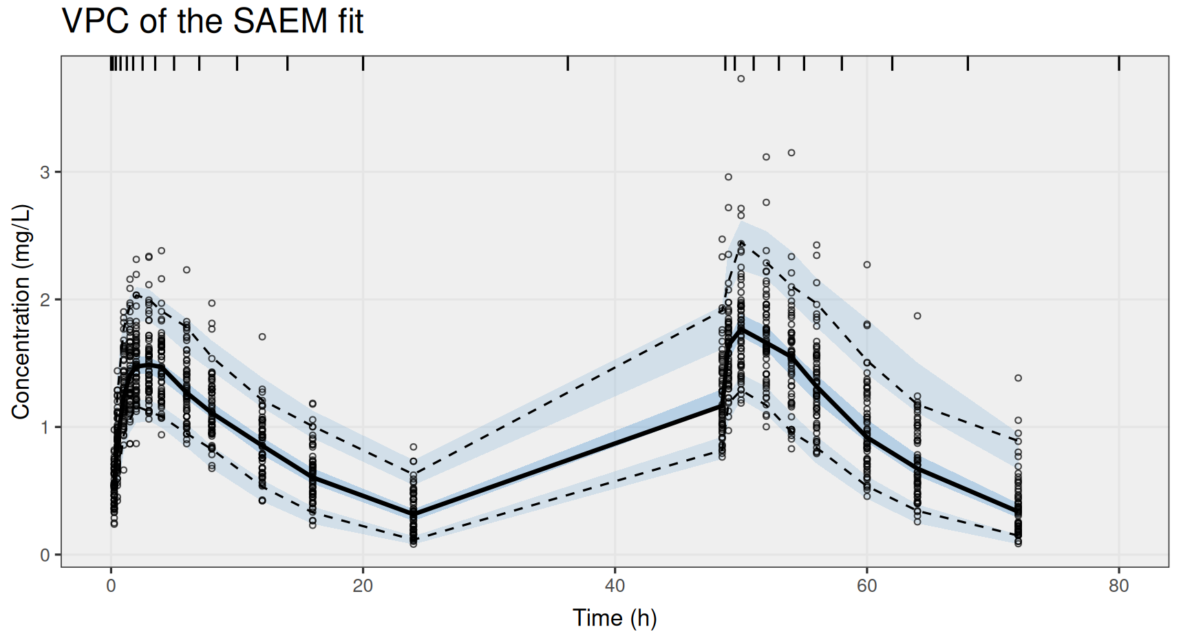

The same applies to augPred(), rxSolve(fit, newEvents) for a new regimen, and the other post-fit tools: you give them one row per dose.

Doses added while solving

The adaptive dosing post showed how a model can add doses during the solve with bolus() and the other evid_() helpers. splitBolus() applies to those doses too. A rescue dose that the model adds to depot is split between depot and slowdepot, just like a dose from the data:

rescue <- function() {
  ini({ka1 <- 1.5; ka2 <- 0.15; fr <- 0.6; cl <- 4; v <- 40})
  model({
    splitBolus(depot, depot, slowdepot)
    f(depot)     <- fr
    f(slowdepot) <- 1 - fr
    d/dt(depot)     <- -ka1 * depot
    d/dt(slowdepot) <- -ka2 * slowdepot
    d/dt(central)   <-  ka1 * depot + ka2 * slowdepot - cl / v * central
    cp <- central / v
    # every 24 h, top up if the trough is below 0.5 mg/L
    if (t > 0 && t %% 24 == 0 && cp < 0.5) {
      bolus(100)
    }
  })
}
resc <- rxSolve(rescue, et(amt = 100, cmt = "depot") |> et(seq(0, 96, by = 0.05)))

resc |>
  as.data.frame() |>
  select(time, depot, slowdepot) |>
  pivot_longer(-time, names_to = "compartment", values_to = "amount") |>
  ggplot(aes(time, amount, color = compartment)) +
  geom_line(linewidth = 1) +
  labs(x = "Time (h)", y = "Amount (mg)",
       title = "Doses the model adds are split 60/40 too")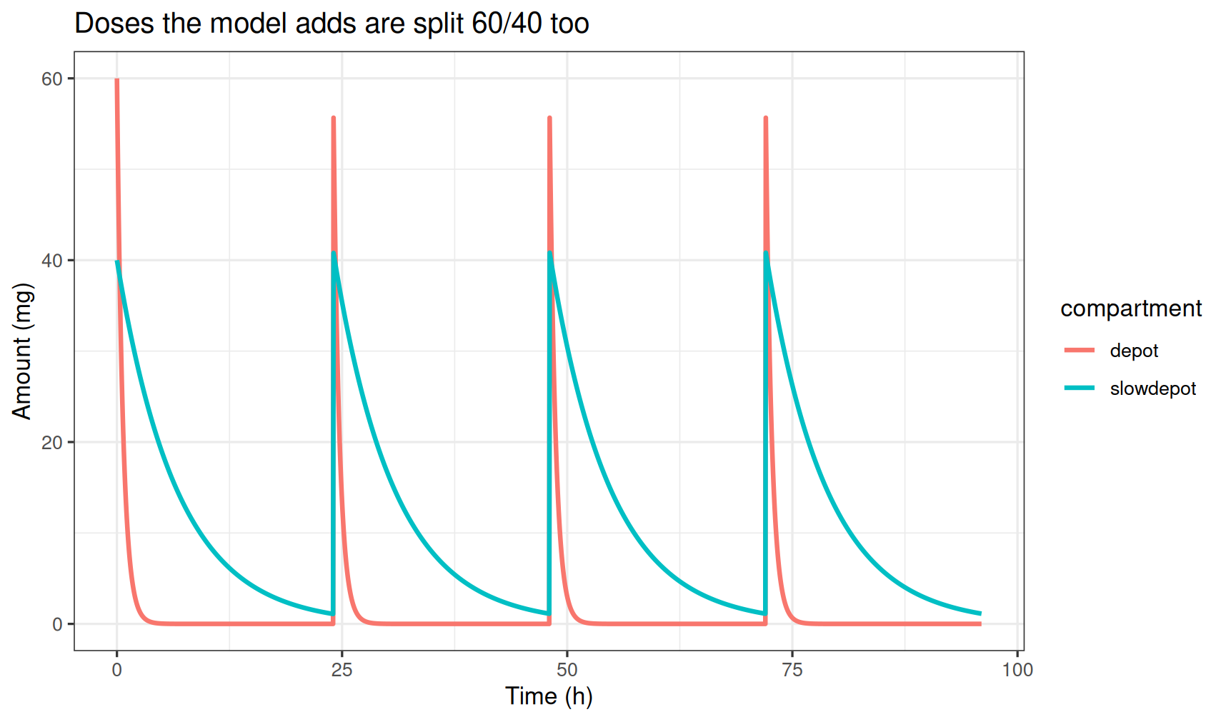

The other three directives work at data-translation time only. Doses added during the solve are not split by splitInfusion(), splitInfusionBolus() or splitBolusInfusion(). If an adaptive model needs to add doses to a split route, use splitBolus().

Summary

• Put one dose row per dose in the data, recorded against a source compartment (depot, sc, …). The source can also be one of the targets.
• Add a splitting directive to model({}) to say where that dose goes: splitBolus(), splitInfusion(), splitInfusionBolus() or splitBolusInfusion().
• Use f() to give each target its share, and alag(), dur() or rate() to give each route its own timing.
• The same model simulates in rxode2 and fits in nlmixr2 (FOCEi, SAEM and the rest), and the post-fit tools apply the split too.

More detail, including the edge cases, is in ?splitBolus, ?splitInfusion, ?`splitInfusionBolus-directive` and ?`splitBolusInfusion-directive`.