rxode2 plotting
By Matthew Fidler in rxode2
February 25, 2025
This month I will focus on rxode2’s plotting functions. I think these
are very useful but not very well known. In general I will focus on
three things: plotting single subjects, plotting multiple subjects and
plotting confidence bands.
Plot functions
rxode2 plotting
Of course discussion of plotting require a model and simulation, so we will use the model from the original tutorial:
library(rxode2)

## Model from rxode2 tutorial
m1 <- rxode2({
  KA <- 2.94E-01
  CL <- 1.86E+01
  V2 <- 4.02E+01
  Q <- 1.05E+01
  V3 <- 2.97E+02
  Kin <- 1
  Kout <- 1
  EC50 <- 200
  ## Added modeled bioavaiblity, duration and rate
  fdepot <- 1
  durDepot <- 8
  rateDepot <- 1250
  C2 <- centr / V2
  C3 <- peri / V3
  d/dt(depot) <- -KA * depot
  f(depot) <- fdepot
  dur(depot) <- durDepot
  rate(depot) <- rateDepot
  d/dt(centr) <- KA * depot - CL * C2 - Q * C2 + Q * C3
  d/dt(peri) <- Q * C2 - Q * C3
  d/dt(eff) <- Kin - Kout * (1 - C2 / (EC50 + C2)) * eff
  eff(0) <- 1
})
rxode2 plotting of single subject solved objects
The first part is plotting a simulation based on a single subject event table:
ev <- et(timeUnits = "hr") %>%
  et(amt = 10000, ii = 12, until = 24) %>%
  et(seq(0, 24, length.out = 100))

s <- rxSolve(m1, ev)

plot(s)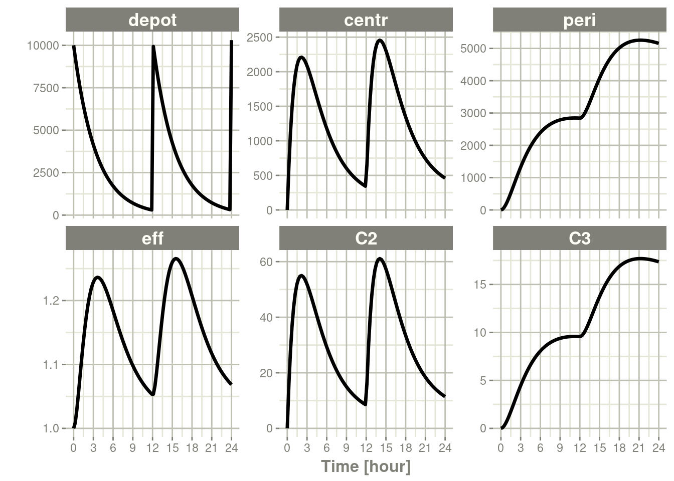
One thing that is very easy to see is that the default plots all the calculated states and parameters in the model.
Often you may not want to see all the plots. For example, if you are
more interested in the C2 concentration, you can subset to C2 by
simply specifying the compartment after the solved object:
plot(s, C2)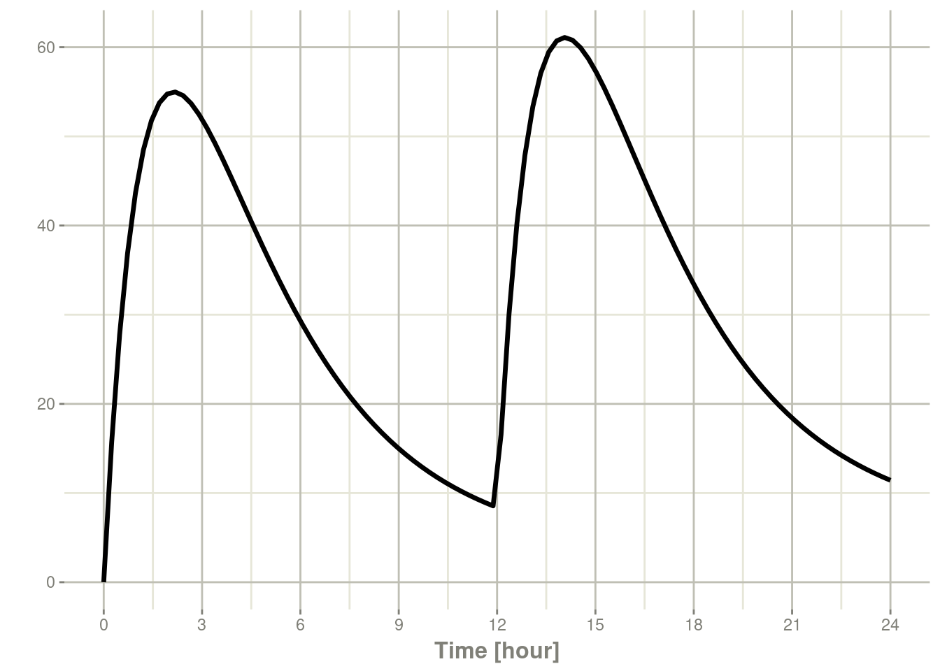
You can specify as many compartments or calculated values as you wish
with this method, for example if you are interested in both C2 and
eff we would have:
plot(s, C2, eff)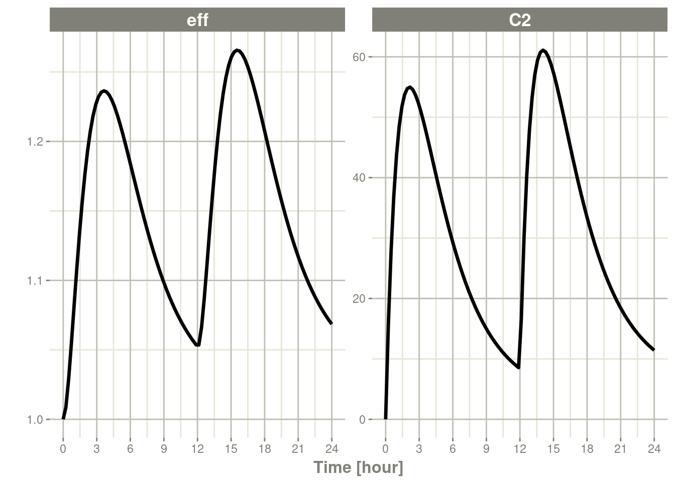
This is one of the most basic types of things that plotting does for
you. As a note, the type of units affects the x-label axis if you
have xgxr installed (for best plotting results this extra tool is
helpful).
withr::with_options(list(rxode2.xgxr = FALSE), {
  plot(s, C2, eff)
})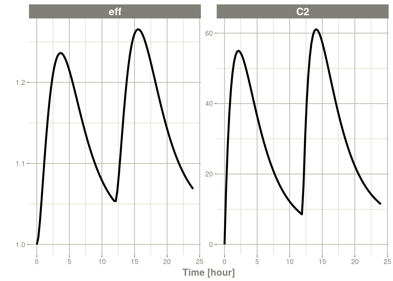
Now the unit ticks are in terms of 5 instead of 3 (which means 24
hours is not even displayed on the plot) by using
xgxr::xgx_scale_x_time_units().
You can also change the axes to be semi-logarithmic with the
log="x", log="y" or log="xy", as documented in the plot()
function:
plot(s, C2, log = "x")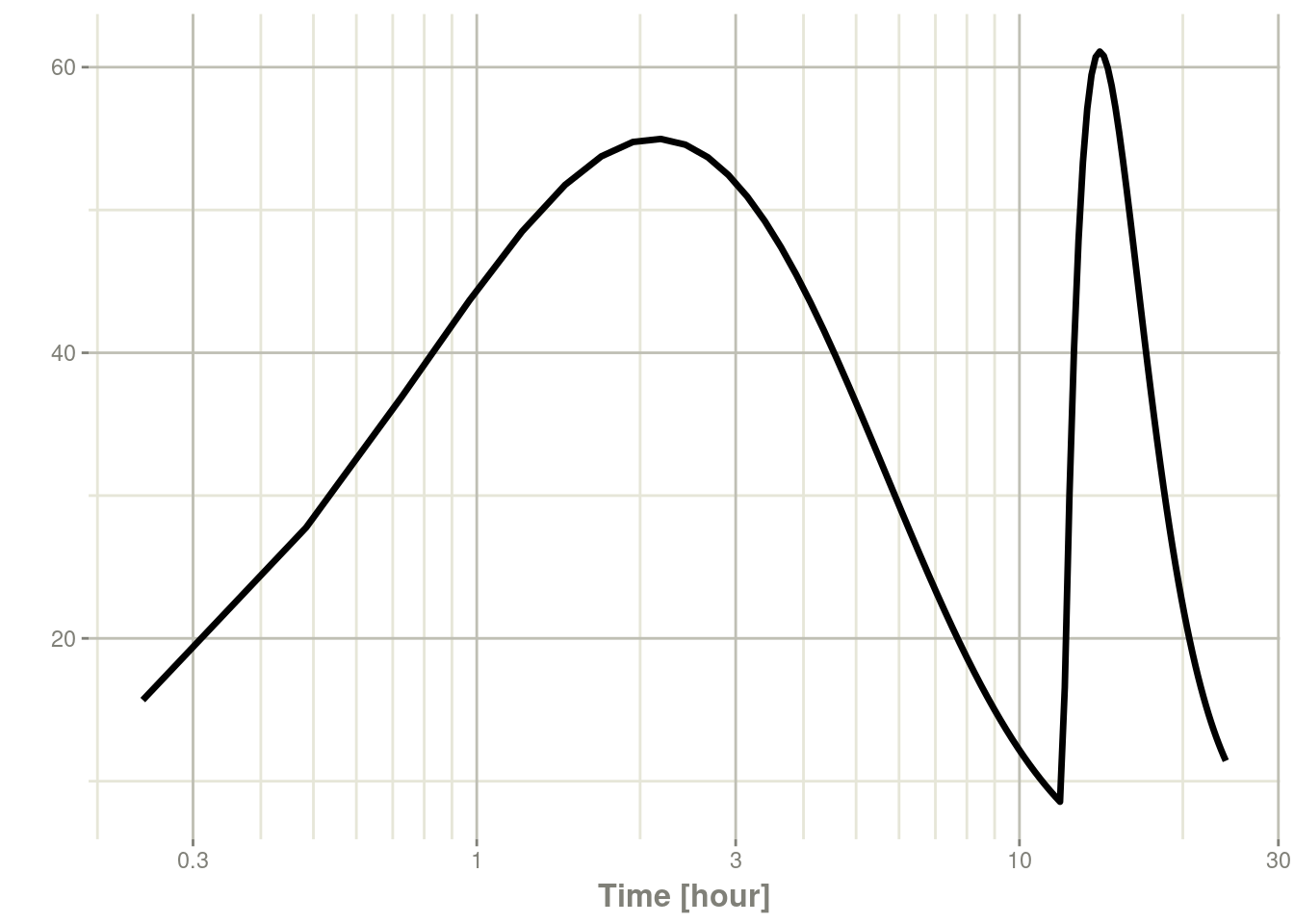
plot(s, C2, log = "y")## Warning in ggplot2::scale_y_log10(..., breaks = breaks, minor_breaks =
## minor_breaks, : log-10 transformation introduced infinite values.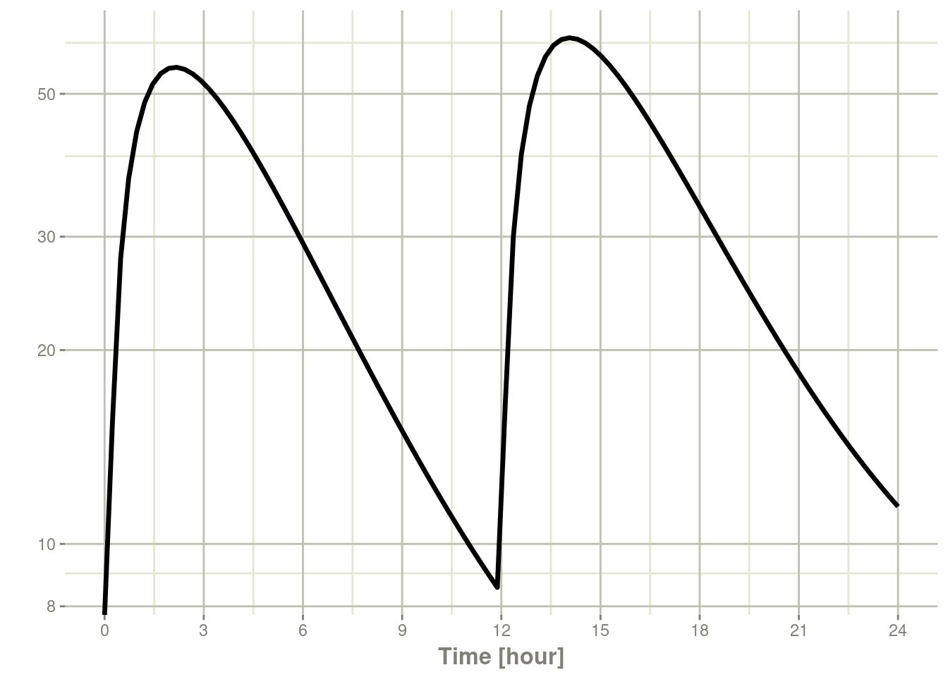
plot(s, C2, log = "xy")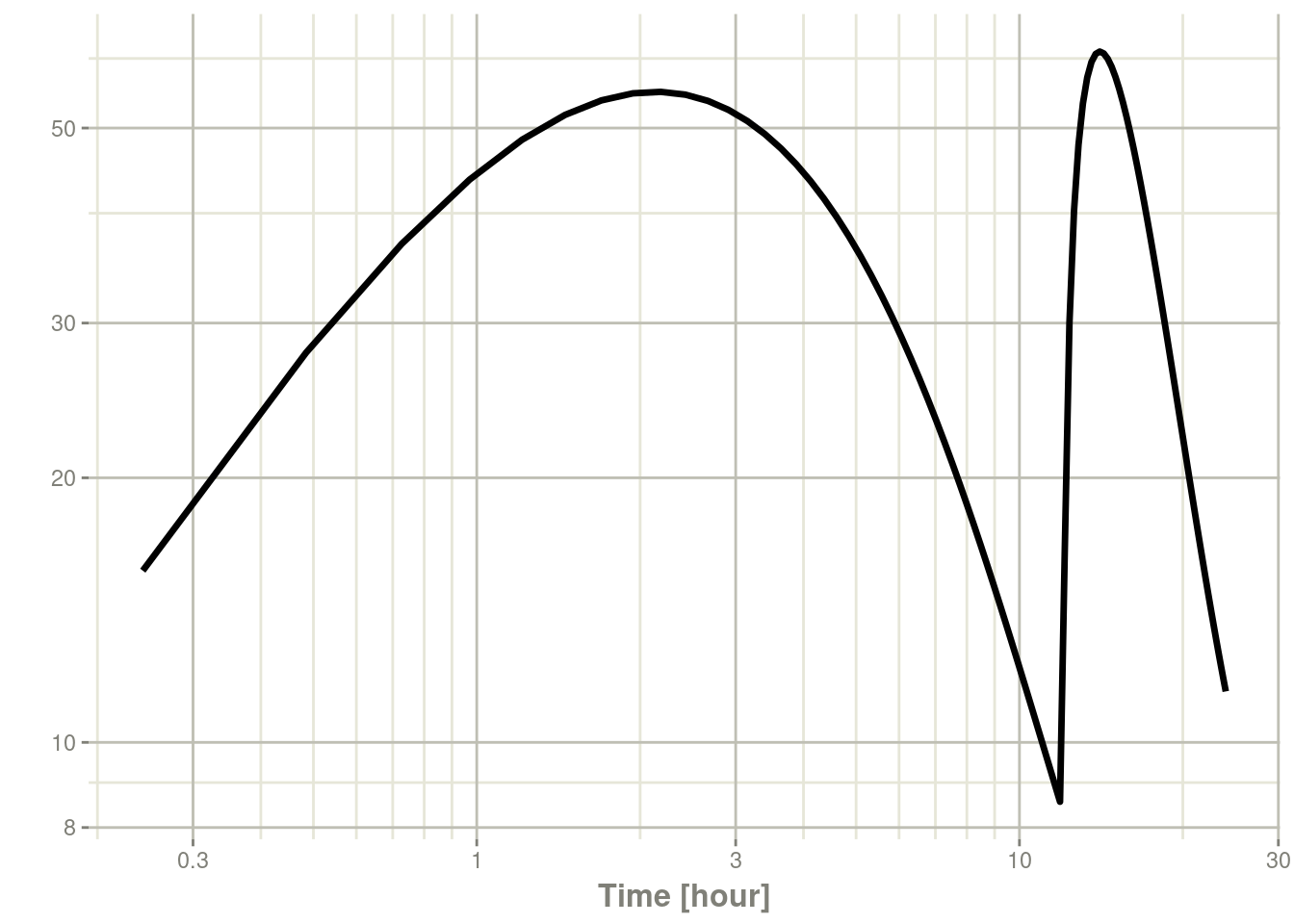
This is done with xgxr::xgx_scale_x_log10() and xgxr::xgx_scale_y_log10()
Currently, the other documented features of plot() are unimplemented
(but may be implemented in the future).
One point is that the return of plot is a ggplot2 object, that
means you can also use ggplot2 types of operations on the object:
library(ggplot2)
plot(s, C2) + xlim(6, 12) + theme_bw()
## Scale for x is already present.
## Adding another scale for x, which will replace the existing scale.## Warning: Removed 75 rows containing missing values or values outside the scale
## range (`geom_line()`).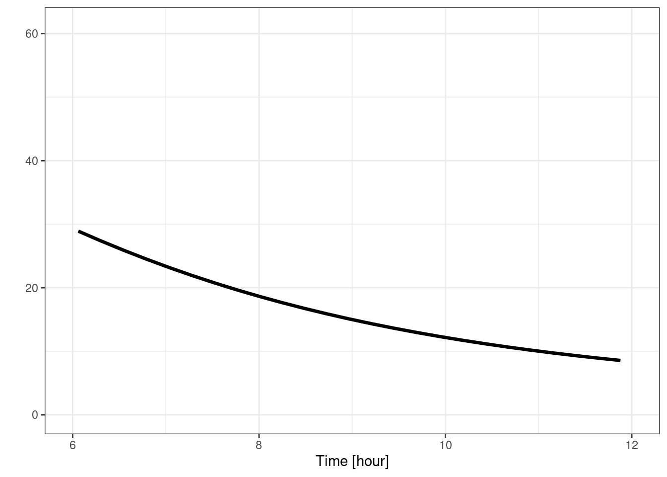
rxode2 plotting of multiple subjects
rxode2 plots multiple subject simulations a bit differently. I will
use model piping to add a log-normal between subject variability on
clearance, and then plot with a few subjects
m2 <- m1 %>%
  model( CL <- 1.86E+01 * exp(eta.Cl)) %>%
  ini(eta.Cl ~ 0.4^2)
## ℹ add between subject variability `eta.Cl` and set estimate to 1## ℹ change initial estimate of `eta.Cl` to `0.16`ev <- et(amount.units = "mg", time.units = "hours") %>%
et(amt = 10000, cmt = "centr", until = 48, ii = 8) %>%
et(0, 36, length.out = 100)
s <- rxSolve(m2, ev, nSub = 3)With only 3 subjects, the subject id is labeled with
ggrepel::geom_label_repel() if ggreple is installed in your system:
plot(s, C2, log="y")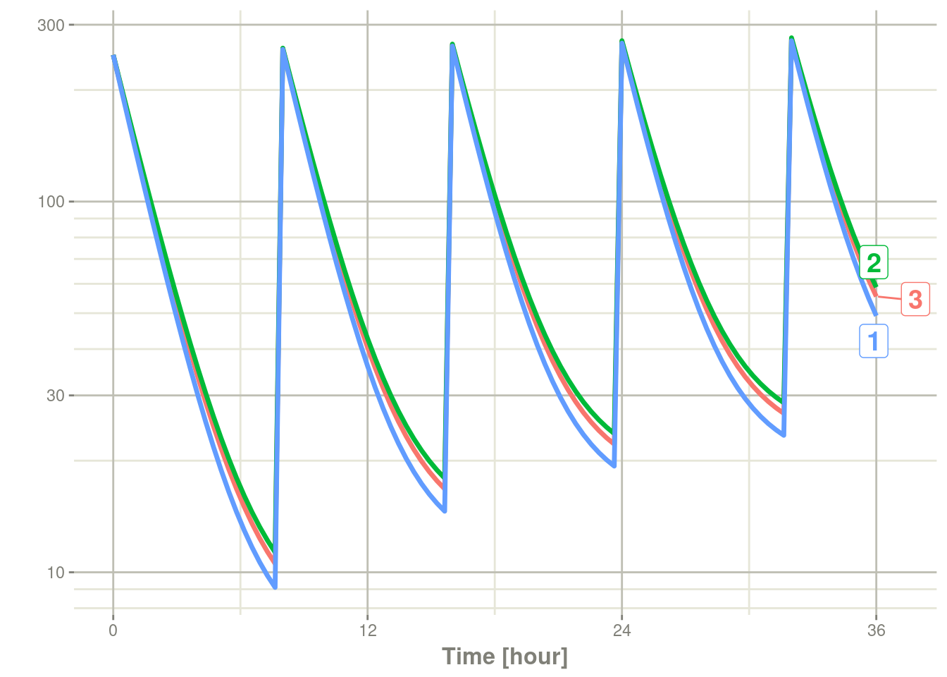
If you get a large number of subjects they become gray spaghetti lines instead:
s <- rxSolve(m2, ev, nSub = 10)

plot(s, C2, log="y")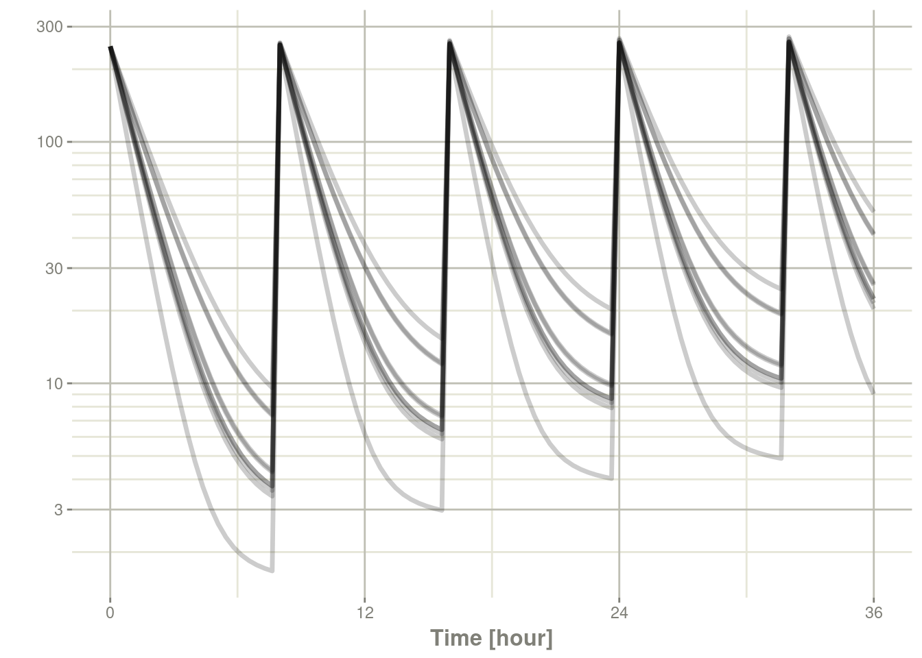
The break-point can be changed with the option rxode2.spaghetti
which defaults to 7 subjects.
options(rxode2.spaghetti=12)
plot(s, C2, log="y")
## Warning: ggrepel: 1 unlabeled data points (too many overlaps). Consider
## increasing max.overlaps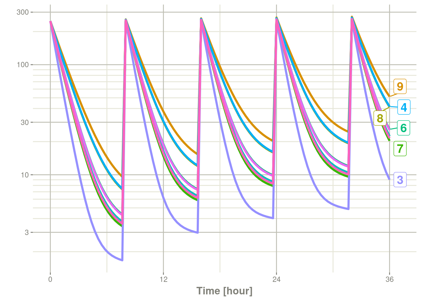
rxode2 summarizing and plotting of multiple subjects confidence intervals
One of the things I do often is to create quantile bands from my simulation.
Continuing from a simple simulation, we have:
s <- rxSolve(m2, ev, nSub=500)

ci <- confint(s, parm=c("eff", "C2"), 0.95)
## ! in order to put confidence bands around the intervals, you need at least 2500 simulations## summarizing data...done# The numeric quantiles from `confint()`
print(ci)## # A tibble: 600 × 5
## time trt p1 eff Percentile
## [h] <fct> <dbl> <dbl> <chr>
## 1 0 eff 0.0250 1 2.5%
## 2 0 eff 0.5 1 50%
## 3 0 eff 0.975 1 97.5%
## 4 0.364 eff 0.0250 1.16 2.5%
## 5 0.364 eff 0.5 1.17 50%
## 6 0.364 eff 0.975 1.18 97.5%
## 7 0.727 eff 0.0250 1.26 2.5%
## 8 0.727 eff 0.5 1.29 50%
## 9 0.727 eff 0.975 1.31 97.5%
## 10 1.09 eff 0.0250 1.29 2.5%
## # ℹ 590 more rowsplot(ci)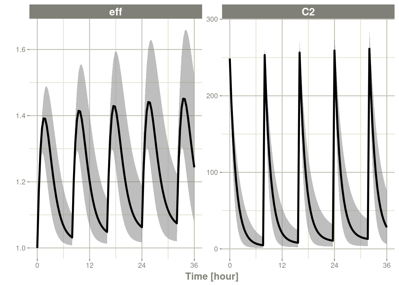
ci <- confint(s, parm=c("eff", "C2"), 0.95)## ! in order to put confidence bands around the intervals, you need at least 2500 simulations
## summarizing data...doneAs mentioned in the notes, with enough simulations you can get a confidence band around the interval.
s <- rxSolve(m2, ev, nSub=2500)

ci <- confint(s, parm=c("eff", "C2"), 0.95)
## summarizing data...done# The numeric confidence intervals:
print(ci)## # A tibble: 600 × 7
## p1 time trt p2.5 p50 p97.5 Percentile
## <dbl> [h] <fct> <dbl> <dbl> <dbl> <fct>
## 1 0.0250 0 eff 1 1 1 2.5%
## 2 0.5 0 eff 1 1 1 50%
## 3 0.975 0 eff 1 1 1 97.5%
## 4 0.0250 0.364 eff 1.16 1.16 1.17 2.5%
## 5 0.5 0.364 eff 1.17 1.17 1.17 50%
## 6 0.975 0.364 eff 1.18 1.18 1.18 97.5%
## 7 0.0250 0.727 eff 1.24 1.26 1.27 2.5%
## 8 0.5 0.727 eff 1.29 1.29 1.30 50%
## 9 0.975 0.727 eff 1.30 1.31 1.31 97.5%
## 10 0.0250 1.09 eff 1.26 1.29 1.32 2.5%
## # ℹ 590 more rowsplot(ci, log="y")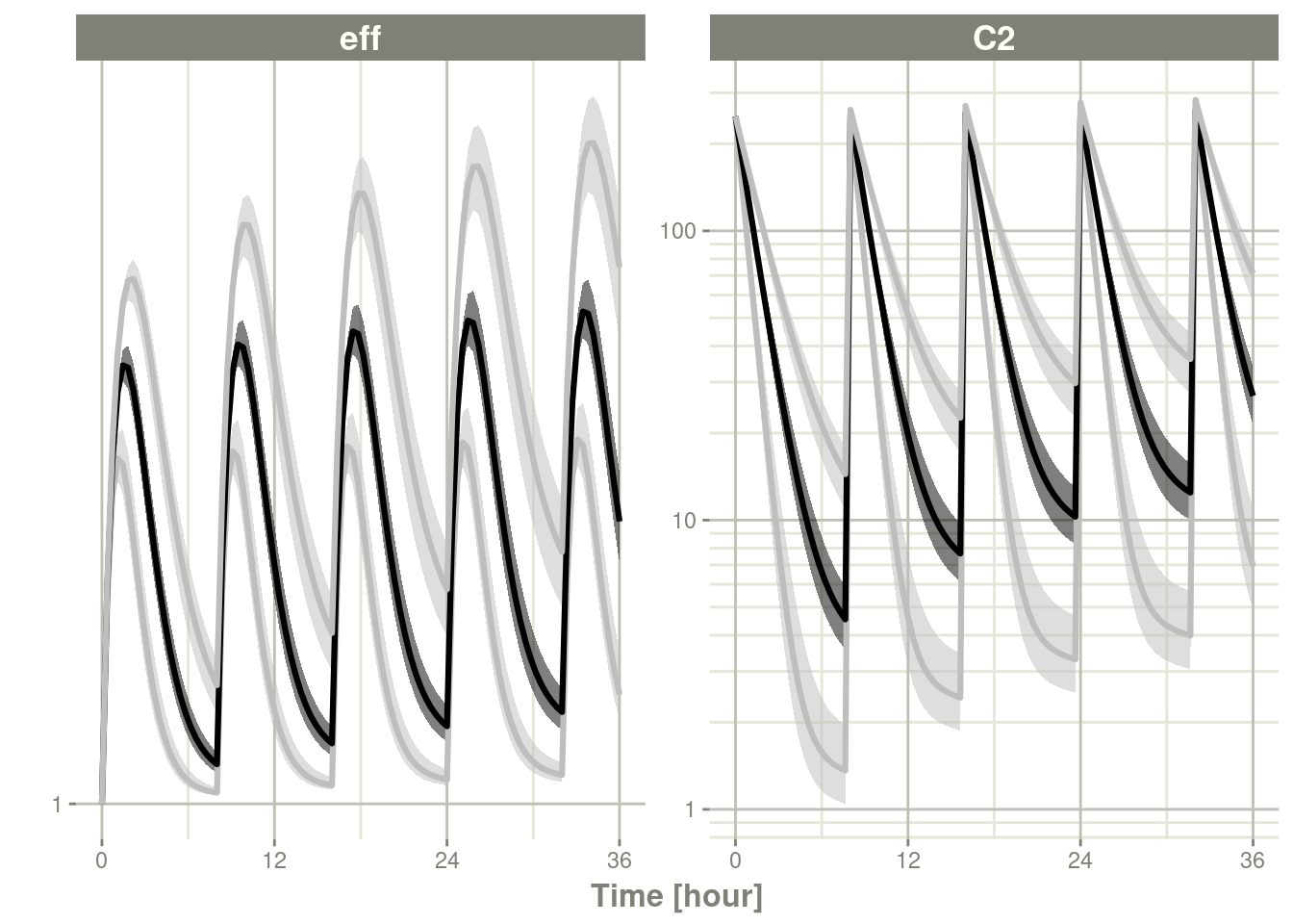
rxode2 stratified quantile intervals
One of the most common tasks that I perform is stratify my simulation by certain sub-groups.
This can be done easily by a rxode2 extension of confint to
stratify with the by argument. An example of this is:
m2 <- m1 %>%
  model( CL <- 1.86E+01 * exp(eta.Cl) + 3*(sex=="Female")) %>%
  ini(eta.Cl ~ 0.4^2)
## ℹ add between subject variability `eta.Cl` and set estimate to 1## ℹ add covariate `sex`## ℹ change initial estimate of `eta.Cl` to `0.16`ev2 <- ev %>% et(id=1:50) %>%
as.data.frame(.) %>%
dplyr::mutate(sex="Male")
ev3 <- ev %>% et(id=51:100) %>%
as.data.frame(.) %>%
dplyr::mutate(sex="Female")
evSex <- rbind(ev2, ev3)
s <- rxSolve(m2, evSex, nStud=500)## [====|====|====|====|====|====|====|====|====|====] 0:00:07# NOTE: by is not a documented in `confint` but can be used
# by a rxode2 solved object
ci <- confint(s, parm=c("eff", "C2"), 0.95, by="sex")## summarizing data...## done# The numeric confidence intervals:
print(ci)## # A tibble: 1,200 × 8
## p1 time trt sex p2.5 p50 p97.5 Percentile
## <dbl> [h] <fct> <fct> <dbl> <dbl> <dbl> <fct>
## 1 0.0250 0 eff Male 1 1 1 2.5%
## 2 0.5 0 eff Male 1 1 1 50%
## 3 0.975 0 eff Male 1 1 1 97.5%
## 4 0.0250 0.364 eff Male 1.16 1.17 1.17 2.5%
## 5 0.5 0.364 eff Male 1.17 1.17 1.17 50%
## 6 0.975 0.364 eff Male 1.18 1.18 1.18 97.5%
## 7 0.0250 0.727 eff Male 1.24 1.26 1.27 2.5%
## 8 0.5 0.727 eff Male 1.29 1.29 1.30 50%
## 9 0.975 0.727 eff Male 1.30 1.31 1.31 97.5%
## 10 0.0250 1.09 eff Male 1.26 1.30 1.32 2.5%
## # ℹ 1,190 more rowsplot(ci)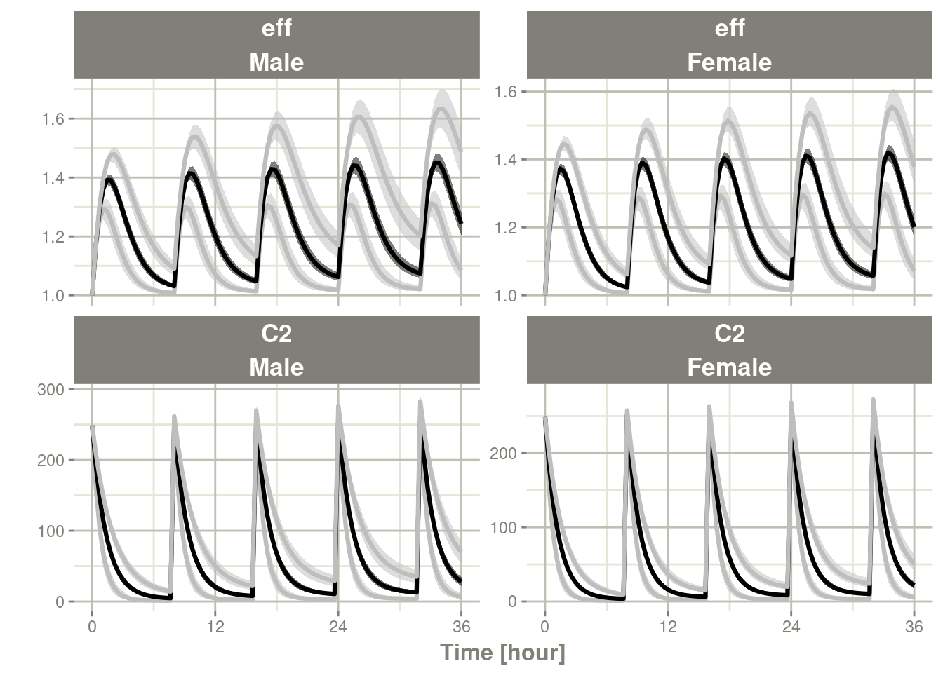
This brings up a couple of points for discussion/understanding.
First, the defaults for confint are a bit different for rxode2
solved objects, this is clearly seen by using the by variable.
Other options other than by are:
ci, in conjunction withlevel, controls levels of the uncertainty in the quantiles or confidence intervals calculatedmean– should the mean values be calculated instead of the quantiles. When this is true instead of thebase::quantile()function, summaries are done withrxode2::meanProbs(), and all the options there are accepted (useT,pred, andn).binom– should binomial values be calculated instead of the binom values. When this is true, instead of using thebase::quantile()function, summaries are done withrxode2::binomProbs()and all the relevant options there are accepted (n,m,ciMethod,pred, etc)
For this blog post I am only focusing on quantiles (perhaps in a later blog post I will cover mean/binom summaries).
ci in confint
By default, the confint is actually the quantiles controlled by
level and ci options, I show extreme options of low and high
ci/levels as well as ci=FALSE to show what each option does.
First we setup the model and the data:
m2 <- m1 %>%
  model( CL <- 1.86E+01 * exp(eta.Cl)) %>%
  ini(eta.Cl ~ 0.4^2)
## ℹ add between subject variability `eta.Cl` and set estimate to 1## ℹ change initial estimate of `eta.Cl` to `0.16`s <- rxSolve(m2, ev, nSub=2500)You can see wider confidence bands in the next plot because the overall levels
is 0.995, but very little variability in the uncertainty of these
bands (since the ci=0.25):
c <- confint(s, parm=c("C2", "eff"), level=.995, ci=.25)## summarizing data...doneplot(c)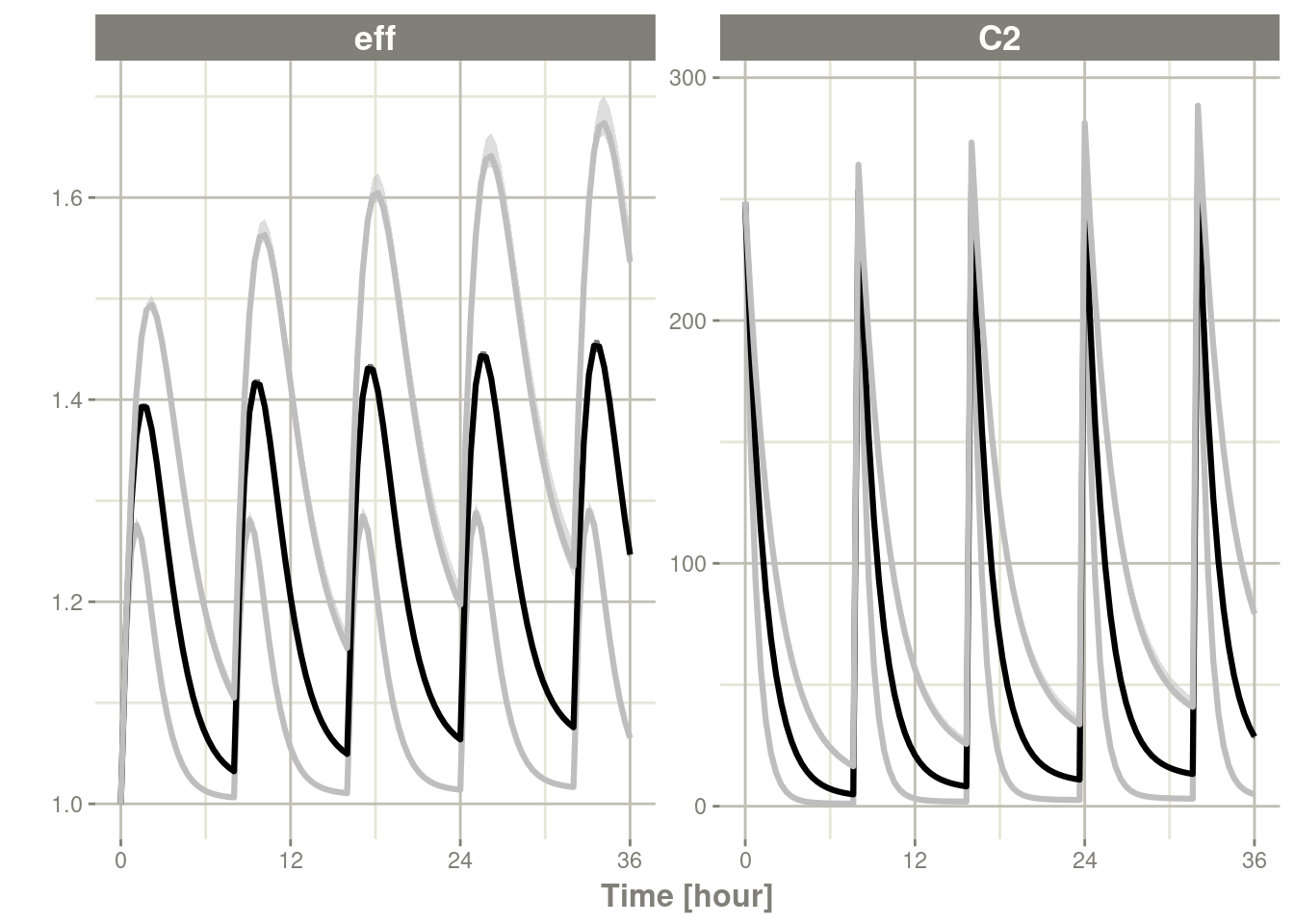
On the other hand, with a level=0.25 the overall confidence bands
are smaller while the confidence around the lines are larger (ci=0.995)
c <- confint(s, parm=c("C2", "eff"), level=.25, ci=.995)## summarizing data...doneplot(c)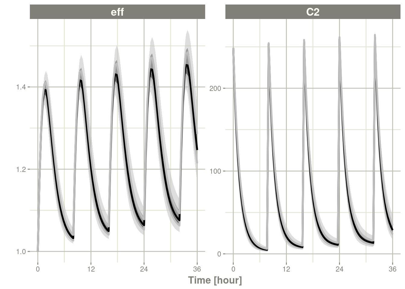
Note that if you specify only level, the ci matches the level
argument:
c <- confint(s, parm=c("C2", "eff"), level=.995)## summarizing data...doneplot(c)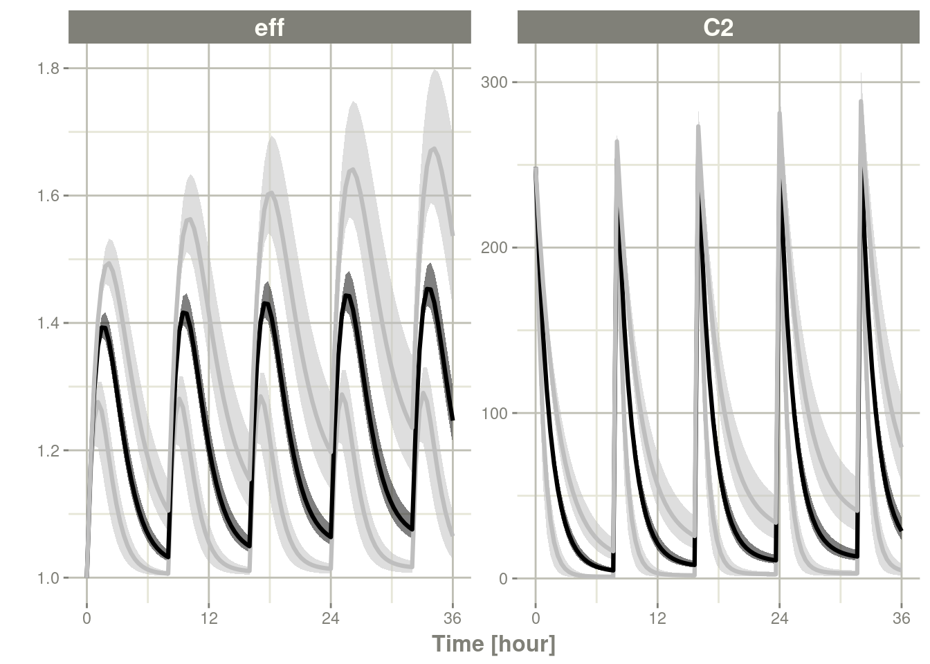
You can also force the simualtion only one quantile calculation by
turning off ci:
c <- confint(s, parm=c("C2", "eff"), level=.995, ci=FALSE)## summarizing data...doneplot(c)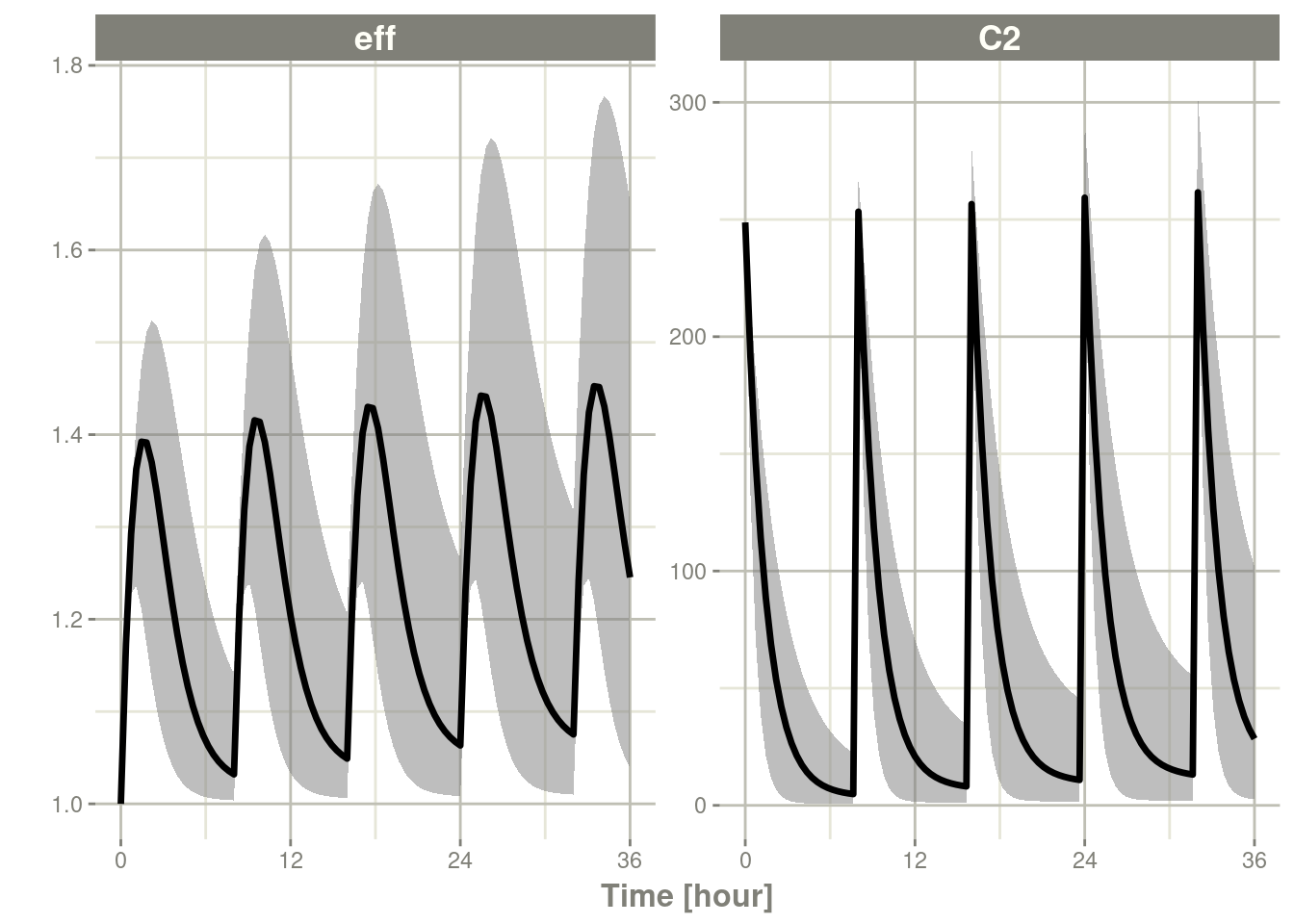
For these confidence bands you can see that the overall level
represents the overall percentiles, while ci represents the
smaller percentiles (which should be illustrated by the above plots).
The for each theoretical study, the quantiles are taken according to
the level. Then these quantiles get confidence around them with
quantiles taken by the values in ci.
For single subject simulations, the number of subjects are split
approximately evenly. For example with 2500 simulations, you would
split the number of studies (nStud) to be round(sqrt(2500)), or
50 with 50 subjects apiece. The first 50 subjects are in
nStud=1, second 50 subjects are in nStud=2, etc.
Other plotting functions
Note there are some other plotting functions in rxode2 like:
rxode2::geom_amt()for showing dosing inrxode2/NONMEMtypes of datasets.rxode2::geom_cens()allows exploration of the censoring data style that is supported bynlmixr2/Monolix.
These may be covered in the future blog and plots from nlmixr2 would
likely be covered later.