RxODE and rxode2

By Matthew Fidler in rxode2

October 12, 2022

`RxODE` vs `rxode2`

Since rxode2 came out recently, I am getting many questions about what is the difference between rxode2 and RxODE.

I think the biggest reason for the question is – is this update going to break all the nice things I already do with RxODE? Or maybe why should I bother to change?

I feel the same way when I have big changes in things I use. For me, I love the ability to pipe and change data with the tidyverse, and similar tools, but hate when they change things that affect my code.

With that in mind, I try to keep changes in behavior small when I modify things like RxODE and rxode2.

In this case, there were much more changes than usual and for that reason I wanted to change the name of the package to rxode2, but I believe most code will run well on either RxODE or rxode2. All changes to rxode2 are listed in the News/Changelog on rxode2’s website and is kept up to date.

What are the changes people may notice?

There are some changes that people will notice and may affect some code. In my opinion these are the big changes:

The options for rxControl and rxSolve are more strict. camelCase is now always used. Old options like add.cov and transit_abs are no longer supported, only addCov is supported. To me this is an annoyance and really makes things a bit easier to remember.
The mnemonic et(rate=model) and et(dur=model) mnemonics have been removed. rate needs to be set to -1 and -2 manually instead.
- This was done because the code for this was a bit cumbersome and hard to maintain
If you use options the prefix changed to rxode2 instead of RxODE.
- This was done so that rxode2 options will not break RxODE options if you wish them to be different.
Running simulations inside of an rxode2 block no longer depends on the number of threads used (a good fix that may be visible to some).
By default the covariates are now added to the dataset (addCov=TRUE) which is different than the behavior of RxODE (addCov=FALSE).
If you use transit compartments by transit_abs this is no longer supported. Instead a special evid=7 is used by all transit compartment doses. This allows mixing with other types of doses into different compartments and better flexibility but will break code.

Things you are unlikely to notice or miss

Various language options (like optionally requiring semi-colons at the end of statements, not allowing <- for instance).

Why bother changing?

Simulating `nlmixr2`/`rxode2` models directly

To me the biggest advantage to using rxode2 is you can simulate from nlmixr2 style models directly. For example, if you wanted to simulate the example nlmixr2 model you can use the following

library(rxode2)
set.seed(42)
rxSetSeed(42)

one.compartment <- function() {
  ini({
    tka <- 0.45 # Log Ka
    tcl <- 1 # Log Cl
    tv <- 3.45    # Log V
    eta.ka ~ 0.6
    eta.cl ~ 0.3
    eta.v ~ 0.1
    add.sd <- 0.7
  })
  # and a model block with the error sppecification and model specification
  model({
    ka <- exp(tka + eta.ka)
    cl <- exp(tcl + eta.cl)
    v <- exp(tv + eta.v)
    d/dt(depot) = -ka * depot
    d/dt(center) = ka * depot - cl / v * center
    cp = center / v
    cp ~ add(add.sd)
  })
}

# Create an event table
et <- et(amt=300) %>%
  et(0,24, by=2) %>%
  et(id=1:12)

# simulate directly from the model
s <- rxSolve(one.compartment, et)

## ℹ parameter labels from comments will be replaced by 'label()'

print(s)

## ── Solved rxode2 object ──
## ── Parameters ($params): ──
## # A tibble: 12 × 8
##    id      tka   tcl    tv add.sd eta.ka  eta.cl   eta.v
##    <fct> <dbl> <dbl> <dbl>  <dbl>  <dbl>   <dbl>   <dbl>
##  1 1      0.45     1  3.45    0.7 -0.206 -1.24   -0.690 
##  2 2      0.45     1  3.45    0.7 -0.392 -0.0876  0.395 
##  3 3      0.45     1  3.45    0.7  0.721  0.383   0.0316
##  4 4      0.45     1  3.45    0.7 -0.502 -0.0715 -0.221 
##  5 5      0.45     1  3.45    0.7  0.791  0.295   0.488 
##  6 6      0.45     1  3.45    0.7 -1.39   0.445  -0.665 
##  7 7      0.45     1  3.45    0.7 -0.846  0.440   0.351 
##  8 8      0.45     1  3.45    0.7 -0.700  0.740   0.275 
##  9 9      0.45     1  3.45    0.7  1.87  -0.158   0.0480
## 10 10     0.45     1  3.45    0.7  0.281 -0.572   0.333 
## 11 11     0.45     1  3.45    0.7 -1.86   0.159   0.450 
## 12 12     0.45     1  3.45    0.7 -0.661  0.199   0.0133
## ── Initial Conditions ($inits): ──
##  depot center 
##      0      0 
## ── First part of data (object): ──
## # A tibble: 156 × 10
##      id  time    ka    cl     v    cp ipredSim   sim      depot center
##   <int> <dbl> <dbl> <dbl> <dbl> <dbl>    <dbl> <dbl>      <dbl>  <dbl>
## 1     1     0  1.28 0.788  15.8   0        0    1.55 300            0 
## 2     1     2  1.28 0.788  15.8  16.3     16.3 16.4   23.4        258.
## 3     1     4  1.28 0.788  15.8  16.1     16.1 15.4    1.82       254.
## 4     1     6  1.28 0.788  15.8  14.6     14.6 14.4    0.142      231.
## 5     1     8  1.28 0.788  15.8  13.3     13.3 12.9    0.0111     210.
## 6     1    10  1.28 0.788  15.8  12.0     12.0 11.9    0.000863   190.
## # … with 150 more rows

plot(s, center)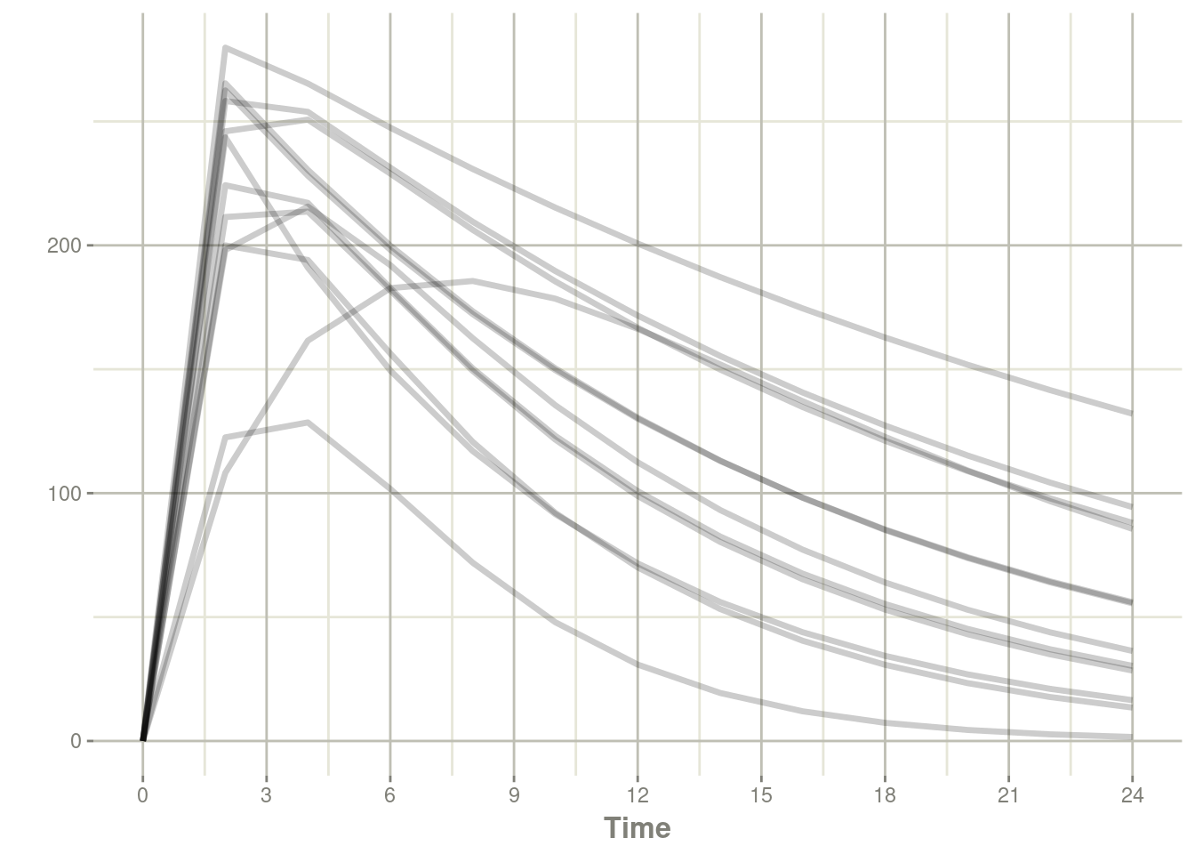

Notice that nlmixr2 was not called (or even required) to simulate this model.

Exploring and changing `nlmixr2`/`rxode2` models directly

One of the nice features is you can change the model by simply changing a line or two of code by a feature called “model piping”. In the model piping included in rxode2 not only does it change your model it tells you how it is changed.

Lets assume you want to explore the impact of between subject variability in the model. You could drop the variability by changing a single line ka <- exp(tka+eta.ka) to ka <- exp(tka). Model piping allows that to occur easily

mod2 <- one.compartment %>%
  model(ka <- exp(tka))

## ℹ parameter labels from comments will be replaced by 'label()'

## ! remove between subject variability `eta.ka`

print(mod2)

##  ── rxode2-based free-form 2-cmt ODE model ────────────────────────────────────── 
##  ── Initalization: ──  
## Fixed Effects ($theta): 
##    tka    tcl     tv add.sd 
##   0.45   1.00   3.45   0.70 
## 
## Omega ($omega): 
##        eta.cl eta.v
## eta.cl    0.3   0.0
## eta.v     0.0   0.1
## 
## States ($state or $stateDf): 
##   Compartment Number Compartment Name
## 1                  1            depot
## 2                  2           center
##  ── μ-referencing ($muRefTable): ──  
##   theta    eta level
## 1   tcl eta.cl    id
## 2    tv  eta.v    id
## 
##  ── Model (Normalized Syntax): ── 
## function() {
##     ini({
##         tka <- 0.45
##         label("Log Ka")
##         tcl <- 1
##         label("Log Cl")
##         tv <- 3.45
##         label("Log V")
##         add.sd <- c(0, 0.7)
##         eta.cl ~ 0.3
##         eta.v ~ 0.1
##     })
##     model({
##         ka <- exp(tka)
##         cl <- exp(tcl + eta.cl)
##         v <- exp(tv + eta.v)
##         d/dt(depot) = -ka * depot
##         d/dt(center) = ka * depot - cl/v * center
##         cp = center/v
##         cp ~ add(add.sd)
##     })
## }

# simulate directly from the model
s <- rxSolve(mod2, et)

print(s)

## ── Solved rxode2 object ──
## ── Parameters ($params): ──
## # A tibble: 12 × 7
##    id      tka   tcl    tv add.sd  eta.cl   eta.v
##    <fct> <dbl> <dbl> <dbl>  <dbl>   <dbl>   <dbl>
##  1 1      0.45     1  3.45    0.7  0.0771  0.782 
##  2 2      0.45     1  3.45    0.7 -0.681  -0.170 
##  3 3      0.45     1  3.45    0.7  0.457  -0.105 
##  4 4      0.45     1  3.45    0.7 -0.336  -0.0738
##  5 5      0.45     1  3.45    0.7 -0.341   0.367 
##  6 6      0.45     1  3.45    0.7  0.244  -0.411 
##  7 7      0.45     1  3.45    0.7  0.212  -0.477 
##  8 8      0.45     1  3.45    0.7 -0.332   0.135 
##  9 9      0.45     1  3.45    0.7 -0.420  -0.439 
## 10 10     0.45     1  3.45    0.7  0.0662 -0.313 
## 11 11     0.45     1  3.45    0.7 -0.561   0.428 
## 12 12     0.45     1  3.45    0.7 -0.146  -0.163 
## ── Initial Conditions ($inits): ──
##  depot center 
##      0      0 
## ── First part of data (object): ──
## # A tibble: 156 × 10
##      id  time    ka    cl     v    cp ipredSim   sim       depot center
##   <int> <dbl> <dbl> <dbl> <dbl> <dbl>    <dbl> <dbl>       <dbl>  <dbl>
## 1     1     0  1.57  2.94  68.8  0        0     1.28 300             0 
## 2     1     2  1.57  2.94  68.8  3.92     3.92  3.53  13.0         270.
## 3     1     4  1.57  2.94  68.8  3.77     3.77  4.16   0.566       259.
## 4     1     6  1.57  2.94  68.8  3.47     3.47  3.58   0.0246      239.
## 5     1     8  1.57  2.94  68.8  3.18     3.18  3.58   0.00107     219.
## 6     1    10  1.57  2.94  68.8  2.92     2.92  2.80   0.0000463   201.
## # … with 150 more rows

plot(s, center)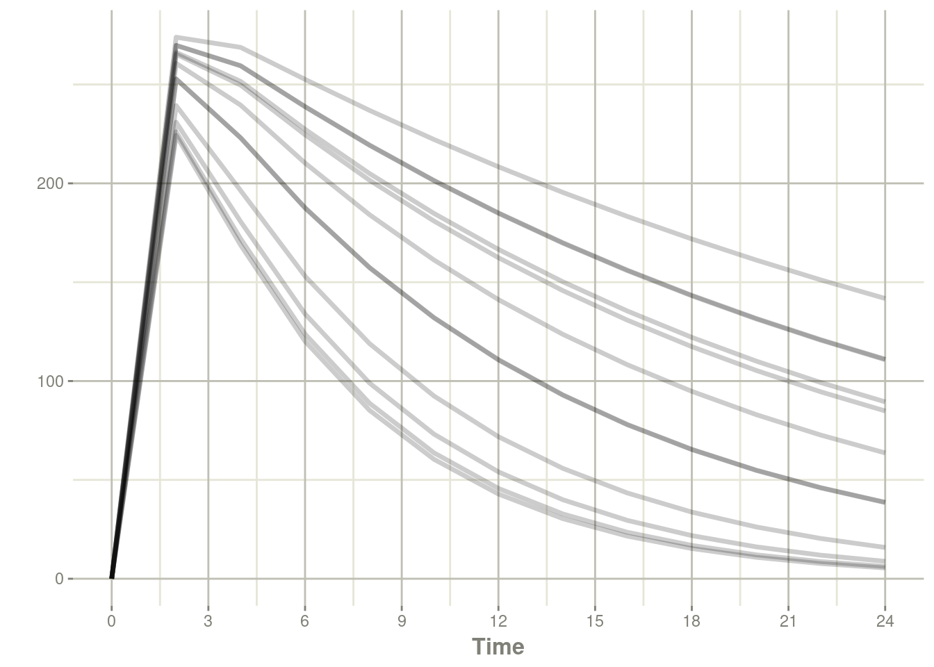

Not surprisingly without between subject variability on the ka component, there is not much difference in absorption between subjects.

What about piping a classic `rxode2` model?

Well when rxode2 2.0.9 is released, you can also pipe a classic rxode2 model, which will change it to a nlmixr2 style model:

mod1 <- rxode2({
  C2 <- centr/V2;
  C3 <- peri/V3;
  d/dt(depot) <- -KA*depot;
  d/dt(centr) <- KA*depot - CL*C2 - Q*C2 + Q*C3;
  d/dt(peri)  <- Q*C2 - Q*C3;
  d/dt(eff)   <- Kin - Kout*(1-C2/(EC50+C2))*eff;
})

mod2 <-  mod1 %>% 
    model(KA <- exp(tka+eta.ka), 
          append=NA) %>% # Prepend a line by append=NA
    ini(tka    = log(0.294), 
        eta.ka = 0.2,
        CL     = 18.6, 
        V2     = 40.2,              # central 
        Q      = 10.5,  
        V3     = 297,               # peripheral
        Kin    = 1, 
        Kout   = 1, 
        EC50   = 200) %>%
    model(eff(0) <- 1)


print(mod2)

s <- rxSolve(mod2, et)

plot(s, centr, eff)

Why wouldn’t I want to switch?

rxode2 requires R 4.0. This is because the BH headers in windows require the R 4.0 toolchains to compile. To remain on CRAN, we needed to have the R 4.0 requirement.

While there may be ways to work-around this in Windows, the new version of rxode2 is not tested with R 4.0, and the old work-around was not straight forward. I cannot recommend you use rxode2 on any of the R versions before R 4.0; it would be too hard to reproduce.

So, in short, if you don’t have R 4.0, I wouldn’t recommend switching.

Posted on:: October 12, 2022

Length:: 8 minute read, 1702 words

Categories:: rxode2

Tags:: new-version

See Also:: nlmixr2 2.1.2/ rxode2 2.1.3; nlmixr2 2.1.0/ rxode2 2.1.1; nonmem2rx and babelmixr2

RxODE vs rxode2