State-Dependent Dosing Properties in rxode2
By Matthew Fidler in rxode2
March 31, 2026
Introduction
A long-standing limitation in rxode2 was that the dosing-modifier
expressions — rate(), dur(), f(), and alag() — could only
reference things that did not depend on state.
If you wanted infusion duration, bioavailability, or lag time to depend
on the current concentration or any other ODE state variable, you
were out of luck.
rxode2 5.0.2 lifts that restriction. All four dosing modifiers, as
well as model-event times (mtime()), can now reference state
variables. The expression is evaluated at the moment the dose fires,
using whatever the system state happens to be at that instant.
This opens the door to more realistic pharmacokinetic models where, for example:
- Infusion rate or duration depends on a patient’s current drug level (e.g., adaptive infusion protocols).
- Bioavailability changes with the concentration of a competing substrate or an enzyme state.
- Absorption lag time varies with gastric emptying driven by another compartment.
- Model event times are triggered by threshold crossings in a state variable.
In this post we walk through each feature with reproducible examples and compare the simulated trajectories against closed-form analytical solutions.
library(rxode2)
library(ggplot2)
library(dplyr)
library(tidyr)
Analytical Helper
All of the rate and duration examples below involve a one-compartment depot that drains with first-order rate constant \(k_a\) and receives a zero-order (constant-rate) infusion. The closed-form solution is:
\[ \text{depot}(t) = \begin{cases} \dfrac{R}{k_a}\bigl(1 - e^{-k_a t}\bigr) & 0 \le t \le D \\[6pt] \dfrac{R}{k_a}\bigl(1 - e^{-k_a D}\bigr)\,e^{-k_a(t-D)} & t > D \end{cases} \]
where \(R\) is the infusion rate and \(D\) is the infusion duration (\(D = \text{amt}/R\) or set directly).
depot_analytic <- function(t, R, D, ka) {
  vapply(t, function(ti) {
    if (ti <= 0) return(0)
    if (ti <= D) {
      (R / ka) * (1 - exp(-ka * ti))
    } else {
      depot_D <- (R / ka) * (1 - exp(-ka * D))
      depot_D * exp(-ka * (ti - D))
    }
  }, numeric(1))
}
State-Dependent Modeled Rate
The idea
rate(depot) <- rate0 + state tells rxode2 that the zero-order
infusion rate into depot is not a fixed parameter but an
expression that includes the ODE variable state.
The rate is evaluated when the dose fires, and the infusion stop-event
is placed at \(t_{\text{dose}} + \text{amt}/R_{\text{eff}}\).
Baseline: state = 0
When the state is zero the expression collapses to the fixed-rate case. This lets us verify that the new code path produces exactly the same answer as before.
mod_rate <- rxode2({
  rate(depot) <- rate0 + state
  d/dt(depot) <- -ka * depot
  d/dt(state) <- 0
})

amt   <- 100
rate0 <- 10
ka    <- 0.5
times <- seq(0, 30, by = 0.25)

et_rate <- et() |>
  et(amt = amt, rate = -1, cmt = "depot") |>
  et(times)

s_rate0 <- rxSolve(mod_rate, et_rate,
                    params = c(rate0 = rate0, ka = ka),
                    inits  = c(state = 0, depot = 0))

R0 <- rate0
D0 <- amt / R0
analytic0 <- depot_analytic(times, R0, D0, ka)

df_rate0 <- data.frame(
  time     = times,
  rxode2   = s_rate0$depot[s_rate0$time %in% times],
  analytic = analytic0
)

ggplot(df_rate0, aes(x = time)) +
  geom_line(aes(y = analytic), colour = "grey40", linewidth = 1.2) +
  geom_point(aes(y = rxode2), colour = "#E74C3C", size = 1.4, alpha = 0.7) +
  labs(title = "State-Dependent Rate — state = 0 (baseline)",
       subtitle = paste0("rate(depot) = ", rate0, " + 0  →  R = ", R0,
                         ", D = ", D0, " h"),
       x = "Time (h)", y = "Depot amount") +
  theme_minimal(base_size = 14)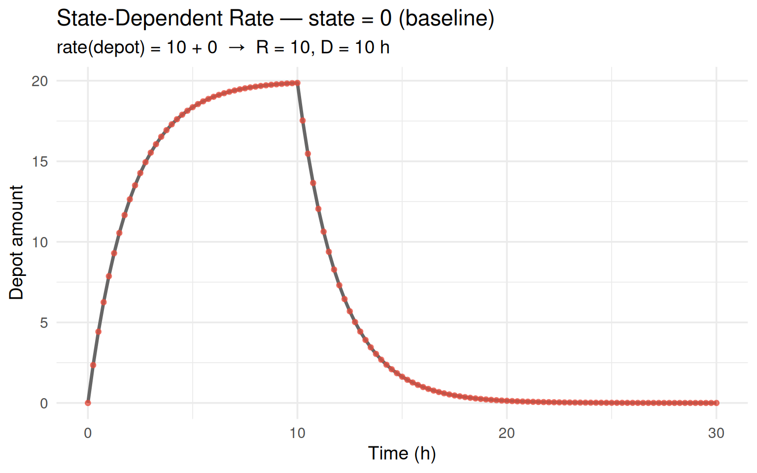
The red dots (simulation) sit exactly on the grey curve (analytical). The new code path reproduces the classical fixed-rate result.
Non-zero state shifts the rate
Setting state to different constant values changes the effective
infusion rate and therefore the duration and peak depot amount.
S0_values <- c(-3, 0, 2, 5)

results_rate <- lapply(S0_values, function(S0) {
  R_eff <- rate0 + S0
  D_eff <- amt / R_eff

  s <- rxSolve(mod_rate, et_rate,
               params = c(rate0 = rate0, ka = ka),
               inits  = c(state = S0, depot = 0))

  data.frame(
    time     = times,
    depot    = s$depot[s$time %in% times],
    analytic = depot_analytic(times, R_eff, D_eff, ka),
    S0       = S0,
    label    = paste0("S0 = ", S0, "  (R = ", R_eff, ", D = ",
                      round(D_eff, 2), " h)")
  )
})

df_rate <- bind_rows(results_rate)

ggplot(df_rate, aes(x = time, colour = label)) +
  geom_line(aes(y = analytic), linewidth = 1.1) +
  geom_point(aes(y = depot), size = 1, alpha = 0.6) +
  labs(title = "State-Dependent Rate — varying initial state",
       subtitle = "rate(depot) <- rate0 + state;   d/dt(state) <- 0",
       x = "Time (h)", y = "Depot amount", colour = NULL) +
  theme_minimal(base_size = 14) +
  theme(legend.position = "top")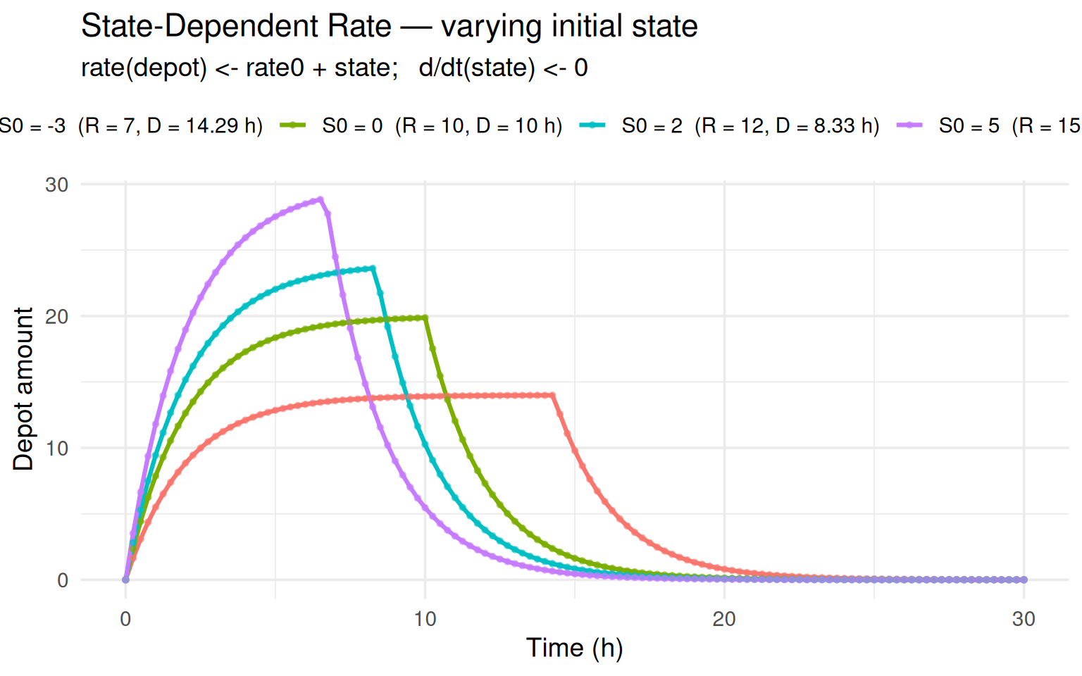
Each trajectory matches its own analytical solution perfectly.
Higher state -> higher rate -> shorter infusion -> lower peak (the drug
is pushed in faster but drains simultaneously).
Consecutive doses with decaying state
When state decays over time each dose sees a different effective
rate. Dose 1 gets the high rate (large state); dose 2 gets a
lower rate because state has decayed.
mod_rate_decay <- rxode2({
  rate(depot) <- rate0 + state
  d/dt(depot) <- -ka * depot
  d/dt(state) <- -kstate * state
})

et_multi <- et() |>
  et(amt = 50, rate = -1, time = 0) |>
  et(amt = 50, rate = -1, time = 15) |>
  et(seq(0, 30, by = 0.25))

s_decay <- rxSolve(mod_rate_decay, et_multi,
                   params = c(rate0 = 5, ka = 0.4, kstate = 0.2),
                   inits  = c(depot = 0, state = 4))

s_nostate <- rxSolve(mod_rate_decay, et_multi,
                     params = c(rate0 = 5, ka = 0.4, kstate = 0.2),
                     inits  = c(depot = 0, state = 0))

df_multi_rate <- bind_rows(
  data.frame(time = s_decay$time,   depot = s_decay$depot,
             Scenario = "state0 = 4 (decaying)"),
  data.frame(time = s_nostate$time, depot = s_nostate$depot,
             Scenario = "state0 = 0 (no shift)")
)

ggplot(df_multi_rate, aes(time, depot, colour = Scenario)) +
  geom_line(linewidth = 0.9) +
  geom_vline(xintercept = c(0, 15), linetype = "dashed", alpha = 0.4) +
  annotate("text", x = 0.5,  y = max(df_multi_rate$depot) * 0.95,
           label = "Dose 1", hjust = 0, size = 3.5) +
  annotate("text", x = 15.5, y = max(df_multi_rate$depot) * 0.95,
           label = "Dose 2", hjust = 0, size = 3.5) +
  labs(title = "Two Doses with Decaying State-Dependent Rate",
       subtitle = "rate(depot) <- rate0 + state;  d/dt(state) <- -kstate * state",
       x = "Time (h)", y = "Depot amount", colour = NULL) +
  theme_minimal(base_size = 14) +
  theme(legend.position = "top")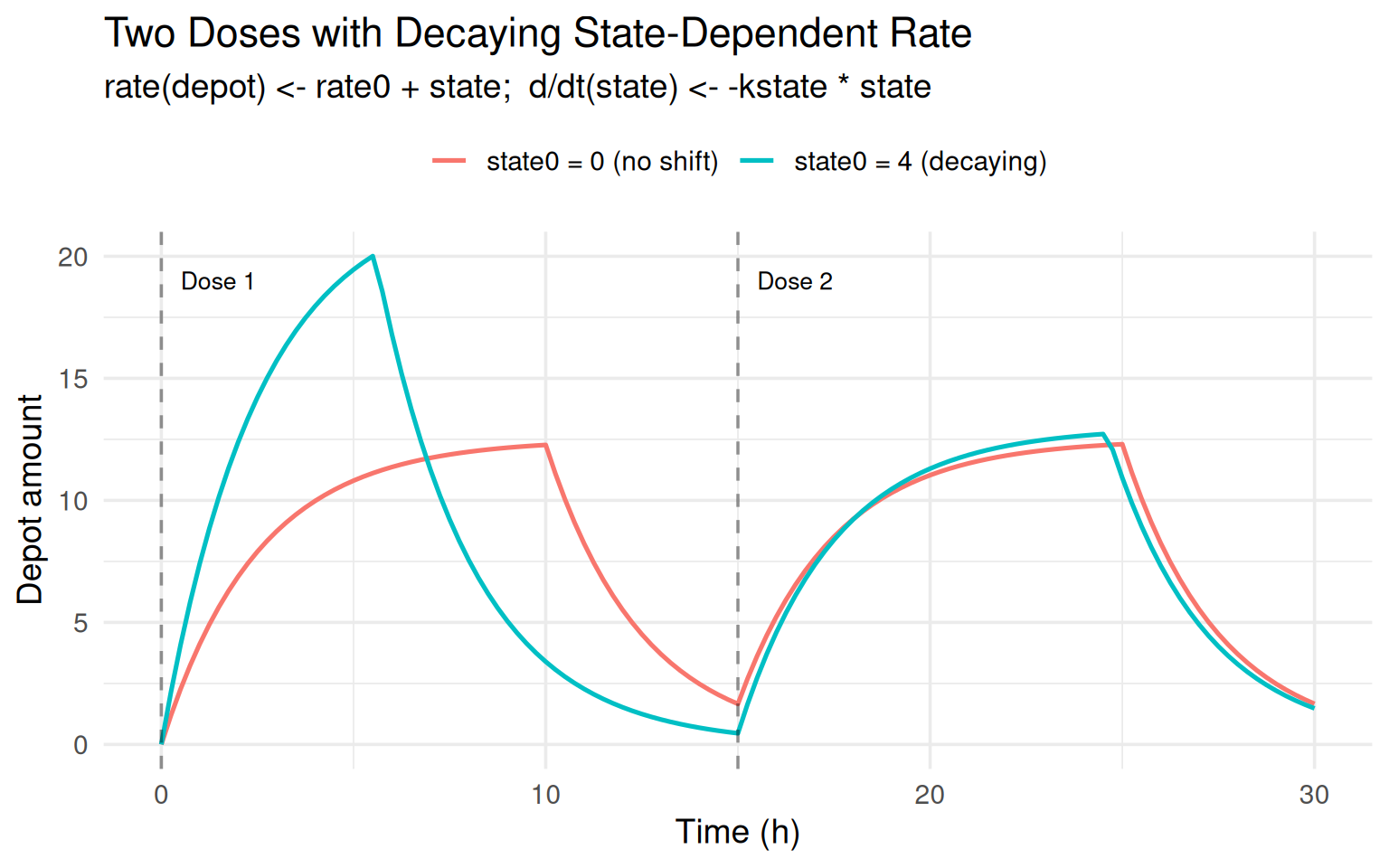
The orange curve is different because dose 1 fires when \(state \approx 4\)
(rate = 9) while dose 2 fires when state has decayed toward zero
(\(rate \approx 5\)).
Per-subject initial state changes the infusion profile
Because the rate expression is evaluated per-subject at the dose time, subjects that start with different compartment values get different infusion profiles automatically.
mod_rate_subj <- rxode2({
  rate(depot) <- central * 0.1 + 1.0
  d/dt(depot) <- -ka * depot
  d/dt(central) <- ka * depot - kel * central
})

et_subj <- et(amt = 100, rate = -1) |> et(seq(0, 24, by = 0.5))

s_c0 <- rxSolve(mod_rate_subj, et_subj, c(ka = 0.5, kel = 0.2),
                 inits = c(depot = 0, central = 0))
s_c5 <- rxSolve(mod_rate_subj, et_subj, c(ka = 0.5, kel = 0.2),
                 inits = c(depot = 0, central = 5))

df_subj_rate <- bind_rows(
  data.frame(time = s_c0$time, central = s_c0$central,
             Subject = "central₀ = 0  (rate = 1.0)"),
  data.frame(time = s_c5$time, central = s_c5$central,
             Subject = "central₀ = 5  (rate = 1.5)")
)

ggplot(df_subj_rate, aes(time, central, colour = Subject)) +
  geom_line(linewidth = 0.9) +
  labs(title = "Per-Subject State-Dependent Rate",
       subtitle = "rate(depot) <- central * 0.1 + 1.0",
       x = "Time (h)", y = "Central amount", colour = NULL) +
  theme_minimal(base_size = 14) +
  theme(legend.position = "top")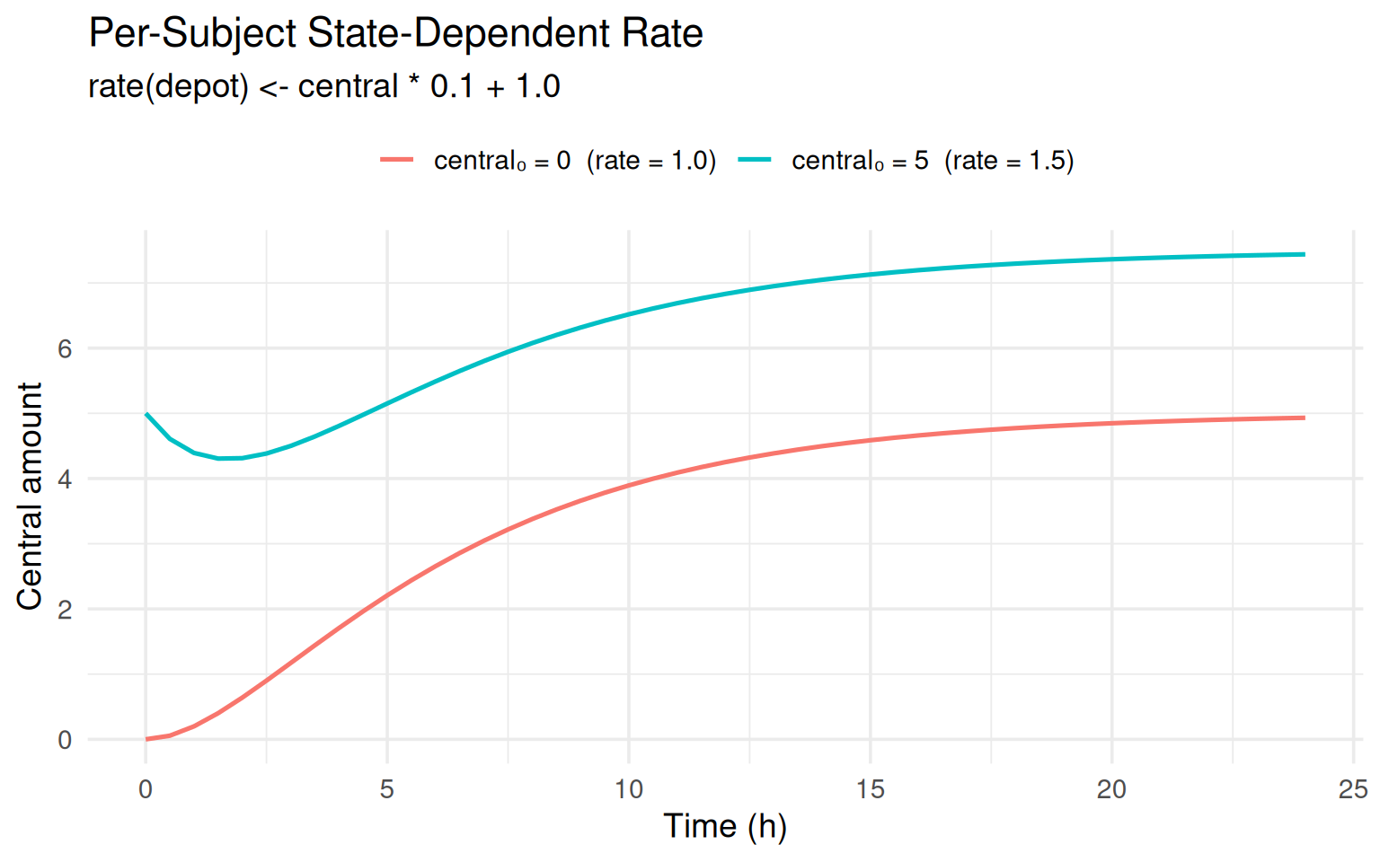
State-Dependent Modeled Duration
The idea
dur(depot) <- dur0 + state sets the infusion duration directly
(rate = -2 in NONMEM convention).
The derived rate is \(R = \text{amt} / (\text{dur0} + \text{state})\).
Baseline and state-shifted duration
mod_dur <- rxode2({
  dur(depot) <- dur0 + state
  d/dt(depot) <- -ka * depot
  d/dt(state) <- 0
})

amt  <- 100
dur0 <- 10
ka   <- 0.5
times <- seq(0, 40, by = 0.25)

et_dur <- et() |>
  et(amt = amt, rate = -2, cmt = "depot") |>
  et(times)

S0_dur <- c(-3, 0, 2, 5)

results_dur <- lapply(S0_dur, function(S0) {
  D_eff <- dur0 + S0
  R_eff <- amt / D_eff

  s <- rxSolve(mod_dur, et_dur,
               params = c(dur0 = dur0, ka = ka),
               inits  = c(state = S0, depot = 0))

  data.frame(
    time     = times,
    depot    = s$depot[s$time %in% times],
    analytic = depot_analytic(times, R_eff, D_eff, ka),
    S0       = S0,
    label    = sprintf("S0 = %d  (D = %g h, R = %.2f)", S0, D_eff, R_eff)
  )
})

df_dur <- bind_rows(results_dur)

ggplot(df_dur, aes(x = time, colour = label)) +
  geom_line(aes(y = analytic), linewidth = 1.1) +
  geom_point(aes(y = depot), size = 0.9, alpha = 0.5) +
  labs(title = "State-Dependent Duration",
       subtitle = "dur(depot) <- dur0 + state;  D = dur0 + S0;  R = amt / D",
       x = "Time (h)", y = "Depot amount", colour = NULL) +
  theme_minimal(base_size = 14) +
  theme(legend.position = "top")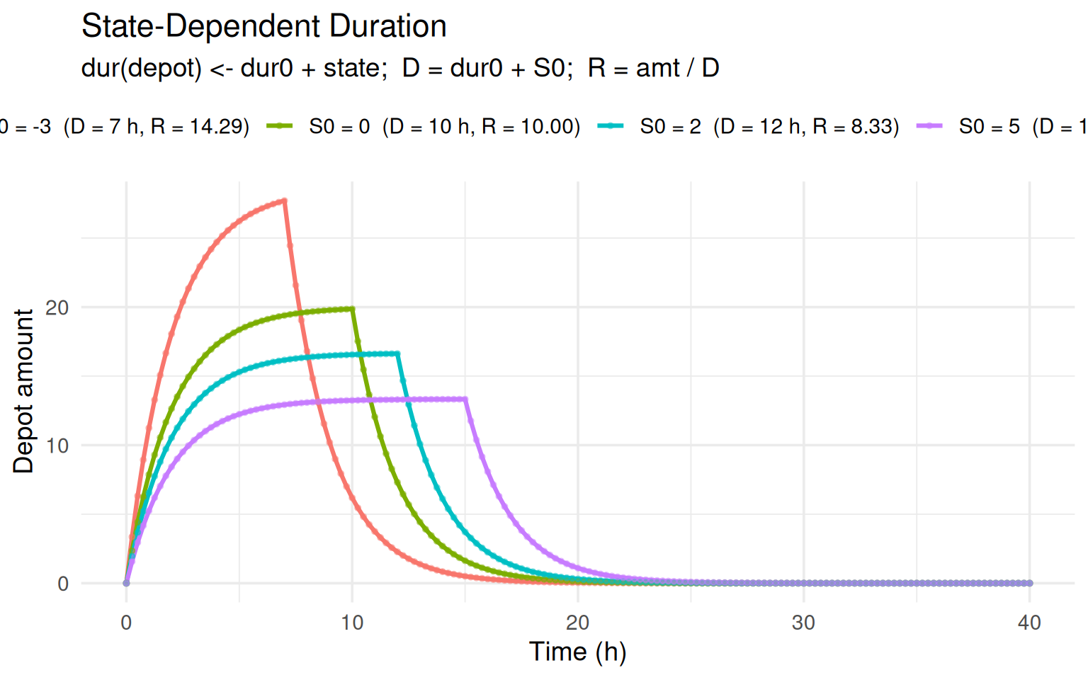
Verifying the exact infusion stop time
A critical check: does the infusion actually stop at exactly \(D = \text{dur0} + \text{state}\)? We sample densely around the expected stop time and compare the depot value at \(t = D\) to the analytical peak.
dur0_check <- 5
ka_check   <- 0.3
S0_check   <- c(0, 3, -1)

stop_check <- lapply(S0_check, function(S0) {
  D <- dur0_check + S0
  R <- amt / D
  fine_times <- sort(unique(c(seq(0, D + 8, by = 0.05), D)))

  et_fine <- et() |>
    et(amt = amt, rate = -2, cmt = "depot") |>
    et(fine_times)

  s <- rxSolve(mod_dur, et_fine,
               params = c(dur0 = dur0_check, ka = ka_check),
               inits  = c(state = S0, depot = 0))

  obs_D      <- s$depot[which.min(abs(s$time - D))]
  expected_D <- (R / ka_check) * (1 - exp(-ka_check * D))

  data.frame(S0 = S0, D = D, R = round(R, 3),
             depot_sim = round(obs_D, 4),
             depot_analytic = round(expected_D, 4),
             match = abs(obs_D - expected_D) < 1e-3)
})

knitr::kable(bind_rows(stop_check),
caption = "Depot at infusion stop time D: simulation vs analytical")| S0 | D | R | depot_sim | depot_analytic | match |
|---|---|---|---|---|---|
| 0 | 5 | 20.0 | 51.7913 | 51.7913 | TRUE |
| 3 | 8 | 12.5 | 37.8868 | 37.8868 | TRUE |
| -1 | 4 | 25.0 | 58.2338 | 58.2338 | TRUE |
Multiple doses with decaying state
mod_dur_decay <- rxode2({
  dur(depot) <- dur0 + state
  d/dt(depot) <- -ka * depot
  d/dt(state) <- -kstate * state
})

et_dur_multi <- et() |>
  et(amt = 50, rate = -2, time = 0) |>
  et(amt = 50, rate = -2, time = 20) |>
  et(seq(0, 35, by = 0.25))

s_dur_decay <- rxSolve(mod_dur_decay, et_dur_multi,
                       params = c(dur0 = 5, ka = 0.4, kstate = 0.2),
                       inits  = c(depot = 0, state = 3))

s_dur_flat  <- rxSolve(mod_dur_decay, et_dur_multi,
                       params = c(dur0 = 5, ka = 0.4, kstate = 0.2),
                       inits  = c(depot = 0, state = 0))

df_dur_multi <- bind_rows(
  data.frame(time = s_dur_decay$time, depot = s_dur_decay$depot,
             Scenario = "state0 = 3 (decaying)"),
  data.frame(time = s_dur_flat$time,  depot = s_dur_flat$depot,
             Scenario = "state0 = 0 (fixed dur)")
)

ggplot(df_dur_multi, aes(time, depot, colour = Scenario)) +
  geom_line(linewidth = 0.9) +
  geom_vline(xintercept = c(0, 20), linetype = "dashed", alpha = 0.4) +
  labs(title = "Multiple Doses with Decaying State-Dependent Duration",
       subtitle = "dur(depot) <- dur0 + state;  d/dt(state) <- -kstate * state",
       x = "Time (h)", y = "Depot amount", colour = NULL) +
  theme_minimal(base_size = 14) +
  theme(legend.position = "top")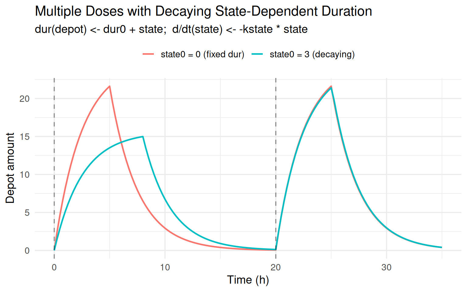
State-Dependent Bioavailability
The idea
f(depot) <- f0 + state means the bioavailable fraction is evaluated
at the moment each dose fires.
For a bolus dose into a mono-exponential depot:
\[ \text{depot}(t) = \text{amt} \cdot (f_0 + S_0)\; e^{-k_a\,t} \]
Single dose — varying state
mod_f <- rxode2({
  f(depot)    <- f0 + state
  d/dt(depot) <- -ka * depot
  d/dt(state) <- 0
})

amt_f <- 100
f0    <- 0.8
ka_f  <- 0.5
times_f <- seq(0, 20, by = 0.25)

et_f <- et() |>
  et(amt = amt_f, cmt = "depot") |>
  et(times_f)

S0_f <- c(-0.2, 0, 0.1, 0.5)

results_f <- lapply(S0_f, function(S0) {
  F_eff <- f0 + S0
  s <- rxSolve(mod_f, et_f,
               params = c(f0 = f0, ka = ka_f),
               inits  = c(state = S0, depot = 0))

  data.frame(
    time     = times_f,
    depot    = s$depot[s$time %in% times_f],
    analytic = amt_f * F_eff * exp(-ka_f * times_f),
    S0       = S0,
    label    = sprintf("S0 = %.1f  (F = %.2f)", S0, F_eff)
  )
})

df_f <- bind_rows(results_f)

ggplot(df_f, aes(x = time, colour = label)) +
  geom_line(aes(y = analytic), linewidth = 1.1) +
  geom_point(aes(y = depot), size = 0.9, alpha = 0.5) +
  labs(title = "State-Dependent Bioavailability — Single Dose",
       subtitle = "f(depot) <- f0 + state;  depot(t) = amt × (f0 + S0) × exp(−ka t)",
       x = "Time (h)", y = "Depot amount", colour = NULL) +
  theme_minimal(base_size = 14) +
  theme(legend.position = "top")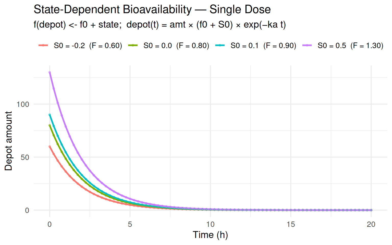
Two doses with decaying state
With a decaying state, the second dose sees a lower bioavailability than the first.
mod_f_decay <- rxode2({
  f(depot)    <- f0 + state
  d/dt(depot) <- -ka * depot
  d/dt(state) <- -kstate * state
})

f0_2     <- 0.8
ka_2     <- 0.5
kstate_2 <- 0.3
amt_2    <- 100
dose_times <- c(0, 5)
times_f2   <- seq(0, 15, by = 0.25)

et_f2 <- et() |>
  et(amt = amt_2, time = 0, cmt = "depot") |>
  et(amt = amt_2, time = 5, cmt = "depot") |>
  et(times_f2)

S0_f2 <- c(0, 0.2, 0.5)

results_f2 <- lapply(S0_f2, function(S0) {
  s <- rxSolve(mod_f_decay, et_f2,
               params = c(f0 = f0_2, ka = ka_2, kstate = kstate_2),
               inits  = c(depot = 0, state = S0))

  # Analytical:  state(t) = S0 * exp(-kstate * t)
  # f at each dose time = f0 + S0 * exp(-kstate * t_d)
  expected <- vapply(times_f2, function(t) {
    contrib <- 0
    for (td in dose_times) {
      if (t >= td) {
        f_td   <- f0_2 + S0 * exp(-kstate_2 * td)
        contrib <- contrib + amt_2 * f_td * exp(-ka_2 * (t - td))
      }
    }
    contrib
  }, numeric(1))

  data.frame(
    time     = times_f2,
    depot    = s$depot[s$time %in% times_f2],
    analytic = expected,
    S0       = S0,
    label    = sprintf("S0 = %.1f", S0)
  )
})

df_f2 <- bind_rows(results_f2)

ggplot(df_f2, aes(x = time, colour = label)) +
  geom_line(aes(y = analytic), linewidth = 1.1) +
  geom_point(aes(y = depot), size = 0.9, alpha = 0.5) +
  geom_vline(xintercept = dose_times, linetype = "dashed", alpha = 0.3) +
  labs(title = "Two Doses with Decaying State-Dependent Bioavailability",
       subtitle = "f(depot) <- f0 + state;  d/dt(state) <- -kstate × state",
       x = "Time (h)", y = "Depot amount", colour = NULL) +
  theme_minimal(base_size = 14) +
  theme(legend.position = "top")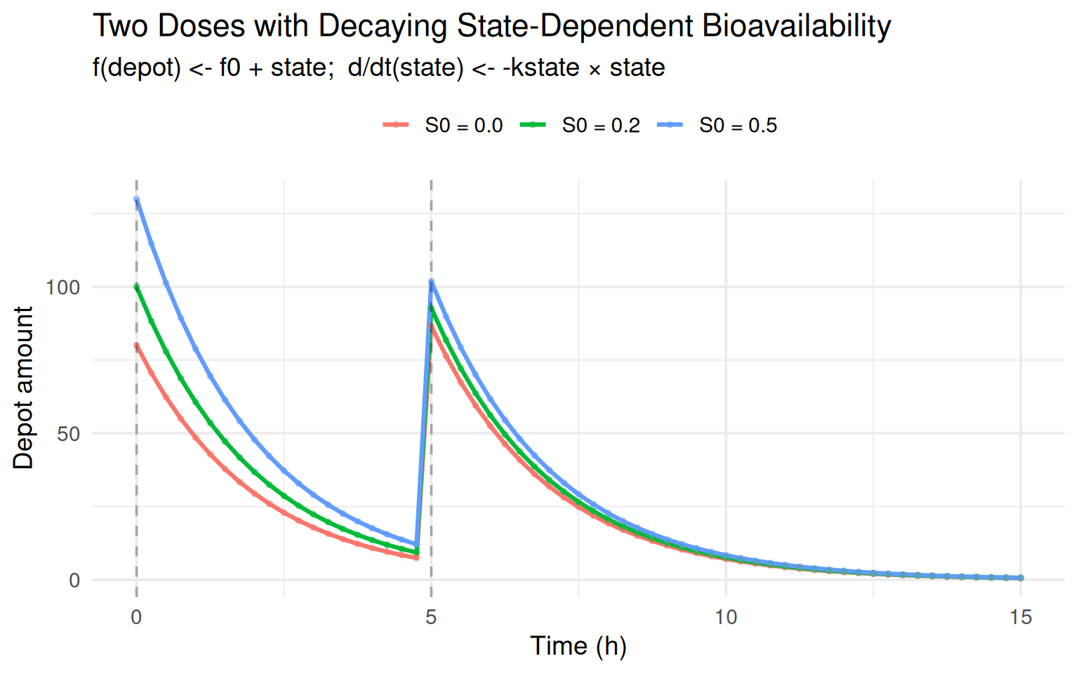
Note how the second dose (dashed line at \(t = 5\)) adds less drug to
the depot when \(S_0 > 0\) because state has partially decayed,
reducing \(f\).
State-Dependent Lag Time (alag)
The idea
alag(depot) <- state_val delays each dose by the current value of
state_val at the scheduled dose time.
A bolus intended for \(t = 0\) actually fires at \(t = \text{state\_val}\).
Constant lag via a state variable
We use d/dt(state_val) <- 0 so the lag is a known constant
and the trajectory is analytically verifiable.
mod_alag <- rxode2({
  alag(depot) <- state_val
  d/dt(depot)     <- -ka * depot
  d/dt(central)   <- ka * depot - kel * central
  d/dt(state_val) <- 0
})

params_alag <- c(ka = 0.5, kel = 0.2)

# Two doses at t = 0 and t = 3
et_alag <- et(amt = 100, time = 0, cmt = "depot") |>
  et(amt = 100, time = 3, cmt = "depot") |>
  et(seq(0, 12, by = 0.25))

lag_values <- c(0, 1, 2)

results_alag <- lapply(lag_values, function(sv) {
  s <- rxSolve(mod_alag, et_alag, params_alag,
               inits = c(depot = 0, central = 0, state_val = sv))

  t_fire1 <- sv
  t_fire2 <- 3 + sv

  analytic <- vapply(s$time, function(t) {
    d <- 0
    if (t >= t_fire1) d <- d + 100 * exp(-0.5 * (t - t_fire1))
    if (t >= t_fire2) d <- d + 100 * exp(-0.5 * (t - t_fire2))
    d
  }, numeric(1))

  data.frame(time = s$time, depot = s$depot,
             analytic = analytic, lag = sv,
             label = paste0("lag = ", sv, " h"))
})

df_alag <- bind_rows(results_alag)

ggplot(df_alag, aes(x = time, colour = label)) +
  geom_line(aes(y = analytic), linewidth = 1.1) +
  geom_point(aes(y = depot), size = 0.9, alpha = 0.5) +
  labs(title = "State-Dependent Lag Time — Constant State",
       subtitle = "alag(depot) <- state_val;  d/dt(state_val) <- 0",
       x = "Time (h)", y = "Depot amount", colour = NULL) +
  theme_minimal(base_size = 14) +
  theme(legend.position = "top")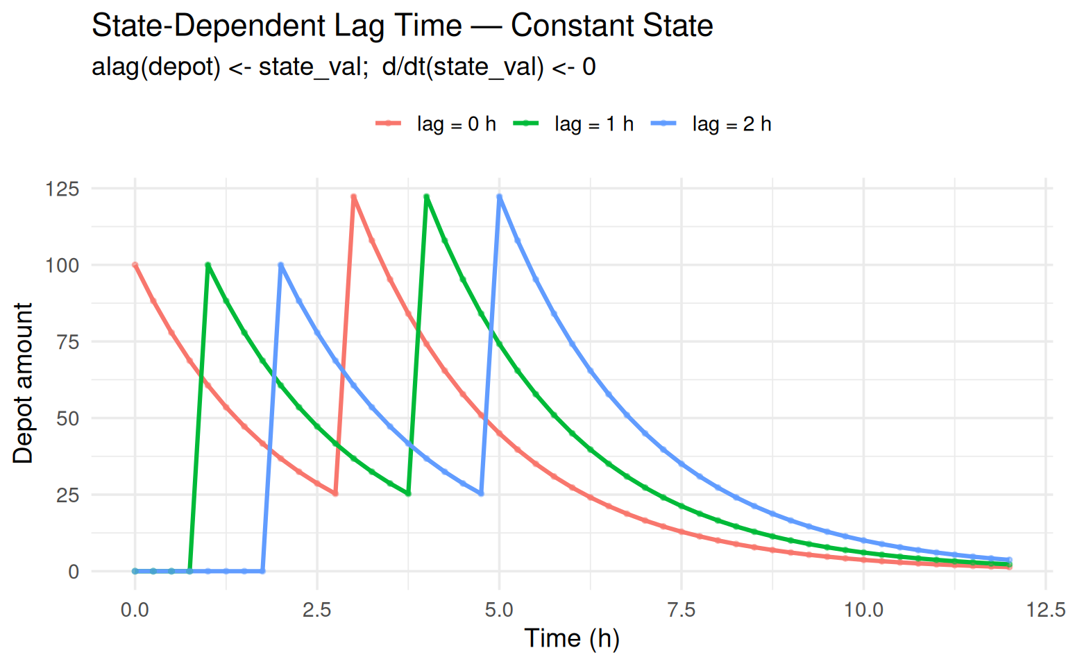
Each dose is shifted rightward by exactly the state_val amount.
Lag depending on a dynamic state
When the lag depends on a compartment that changes over time, each dose gets a different effective lag.
mod_alag_dyn <- rxode2({
  alag(depot) <- central * 0.1
  d/dt(depot)   <- -ka * depot
  d/dt(central) <- ka * depot - kel * central
})

et_alag_dyn <- et() |>
  et(amt = 100, time = 0) |>
  et(amt = 100, time = 6) |>
  et(seq(0, 24, by = 0.25))

s_lag0 <- rxSolve(mod_alag_dyn, et_alag_dyn,
                  c(ka = 0.5, kel = 0.2),
                  inits = c(depot = 0, central = 0))

s_lag5 <- rxSolve(mod_alag_dyn, et_alag_dyn,
                  c(ka = 0.5, kel = 0.2),
                  inits = c(depot = 0, central = 5))

df_alag_dyn <- bind_rows(
  data.frame(time = s_lag0$time, central = s_lag0$central,
             Subject = "central0 = 0  (lag = 0 h)"),
  data.frame(time = s_lag5$time, central = s_lag5$central,
             Subject = "central0 = 5  (lag = 0.5 h)")
)

ggplot(df_alag_dyn, aes(time, central, colour = Subject)) +
  geom_line(linewidth = 0.9) +
  labs(title = "Dynamic State-Dependent Lag Time",
       subtitle = "alag(depot) <- central × 0.1",
       x = "Time (h)", y = "Central amount", colour = NULL) +
  theme_minimal(base_size = 14) +
  theme(legend.position = "top")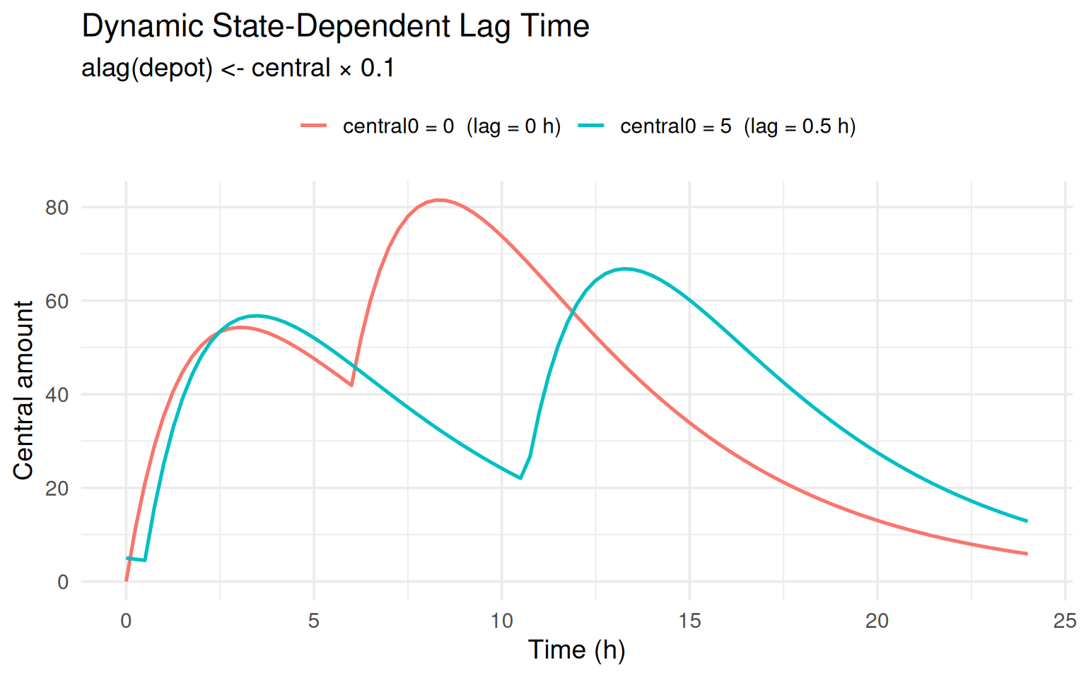
The subject starting with central = 5 has a 0.5 h lag on the first
dose, visibly delaying the rise in central concentrations.
Combining Features: Lag + Duration
Dosing modifiers compose. Here we combine a fixed lag with a state-dependent duration to show that the infusion-stop event is placed at the correct absolute time: \(t_{\text{stop}} = t_{\text{dose}} + \text{lag} + \text{dur}\).
mod_combo <- rxode2({
  alag(depot) <- 0.5
  dur(depot)  <- central * 0.1 + 1.0
  d/dt(depot)   <- -ka * depot
  d/dt(central) <- ka * depot - kel * central
})

et_combo <- et(amt = 100, rate = -2) |> et(seq(0, 24, by = 0.25))

s_combo <- rxSolve(mod_combo, et_combo,
                   c(ka = 0.5, kel = 0.2),
                   inits = c(depot = 0, central = 3))

s_combo0 <- rxSolve(mod_combo, et_combo,
                    c(ka = 0.5, kel = 0.2),
                    inits = c(depot = 0, central = 0))

df_combo <- bind_rows(
  data.frame(time = s_combo$time, depot = s_combo$depot,
             central = s_combo$central,
             Scenario = "central₀ = 3  (lag 0.5 h, dur ≈ 1.3 h)"),
  data.frame(time = s_combo0$time, depot = s_combo0$depot,
             central = s_combo0$central,
             Scenario = "central₀ = 0  (lag 0.5 h, dur = 1.0 h)")
)

p_combo_depot <- ggplot(df_combo, aes(time, depot, colour = Scenario)) +
  geom_line(linewidth = 0.9) +
  labs(title = "Combined Lag + State-Dependent Duration — Depot",
       subtitle = "alag(depot) <- 0.5;  dur(depot) <- central × 0.1 + 1.0",
       x = "Time (h)", y = "Depot amount", colour = NULL) +
  theme_minimal(base_size = 14) +
  theme(legend.position = "top")

p_combo_central <- ggplot(df_combo, aes(time, central, colour = Scenario)) +
  geom_line(linewidth = 0.9) +
  labs(title = "Combined Lag + State-Dependent Duration — Central",
       x = "Time (h)", y = "Central amount", colour = NULL) +
  theme_minimal(base_size = 14) +
  theme(legend.position = "top")

p_combo_depot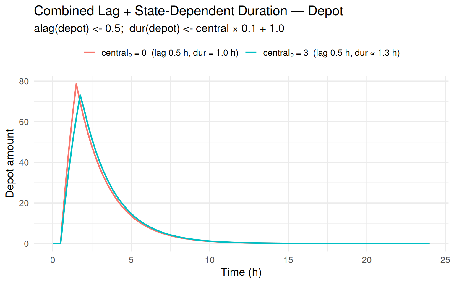
p_combo_central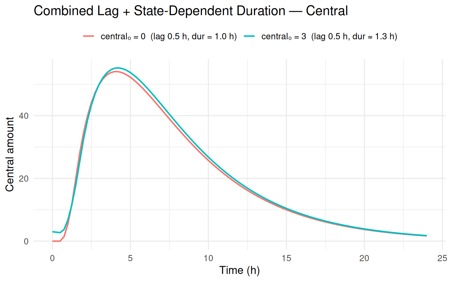
The subject with central₀ = 3 has a slightly longer infusion
duration ($0.1 + 1 = 1.3$ h) compared to the baseline
($1.0$ h).
Both subjects share the same 0.5 h absorption lag.
The plots confirm that the stop-event is placed correctly:
the depot rises only after the lag, and the infusion ends at
\[t = 0 + 0.5 + \text{dur}\].
State-Dependent Model Event Times (mtime)
The idea
mtime() inserts an extra observation/solver-restart time into the
integration grid.
Previously the argument had to be a constant or parameter expression.
Now it can reference state variables, enabling event times that depend
on the evolving system.
A practical use case is triggering a covariate shift (e.g., enzyme induction onset) at a time that depends on cumulative drug exposure.
mod_mtime <- rxode2({
  # Model event time depends on a state variable
  # state decays; mtime fires at t = 2 + state (evaluated at init)
  mtime(mt) <- 2 + state

  # Effect switches on at the model event time
  eff <- ifelse(time >= mt, 1, 0)

  d/dt(depot)   <- -ka * depot
  d/dt(central) <- ka * depot - kel * central * (1 + 0.5 * eff)
  d/dt(state)   <- -kstate * state
})


et_mt <- et(amt = 100) |> et(seq(0, 24, by = 0.1))

s_mt0 <- rxSolve(mod_mtime, et_mt,
                 c(ka = 1.0, kel = 0.2, kstate = 0.1),
                 inits = c(depot = 0, central = 0, state = 0))

s_mt3 <- rxSolve(mod_mtime, et_mt,
                 c(ka = 1.0, kel = 0.2, kstate = 0.1),
                 inits = c(depot = 0, central = 0, state = 3))

s_mt6 <- rxSolve(mod_mtime, et_mt,
                 c(ka = 1.0, kel = 0.2, kstate = 0.1),
                 inits = c(depot = 0, central = 0, state = 6))

df_mtime <- bind_rows(
  data.frame(time = s_mt0$time, central = s_mt0$central,
             Scenario = "state0 = 0  (mtime = 2 h)"),
  data.frame(time = s_mt3$time, central = s_mt3$central,
             Scenario = "state0 = 3  (mtime = 5 h)"),
  data.frame(time = s_mt6$time, central = s_mt6$central,
             Scenario = "state0 = 6  (mtime = 8 h)")
)

ggplot(df_mtime, aes(time, central, colour = Scenario)) +
  geom_line(linewidth = 0.9) +
  geom_vline(xintercept = c(2, 5, 8), linetype = "dashed", alpha = 0.3) +
  annotate("text", x = c(2.3, 5.3, 8.3),
           y = rep(max(df_mtime$central) * 0.95, 3),
           label = c("mtime=2", "mtime=5", "mtime=8"),
           size = 3, hjust = 0) +
  labs(title = "State-Dependent Model Event Times",
       subtitle = "mtime(mt) <- 2 + state;  eff switches on at mt",
       x = "Time (h)", y = "Central amount", colour = NULL) +
  theme_minimal(base_size = 14) +
  theme(legend.position = "top")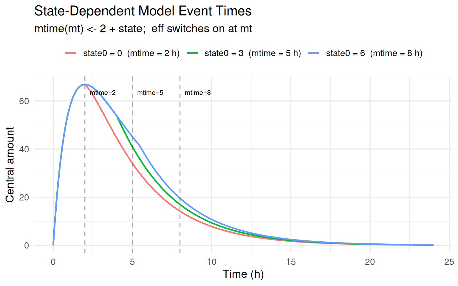
The dashed vertical lines mark the model event time for each scenario.
Higher initial state pushes the effect onset later, resulting in
higher peak concentrations (the enhanced elimination kicks in later).
Summary of New Capabilities
The table below summarizes what is now possible with state-dependent dosing properties:
| Feature | NONMEM Analog | When Evaluated | Key Behaviour |
|---|---|---|---|
| rate(cmt) | RATE = -1 with state-dep expression | At dose firing time | Infusion stop re-sorted; R = expr at dose time |
| dur(cmt) | RATE = -2 with state-dep expression | At dose firing time | Duration = expr at dose time; R = amt/dur |
| f(cmt) | F1 depending on state | At dose firing time | Effective amount = amt × f(state) |
| alag(cmt) | ALAG1 depending on state | At dose sorting / firing time | Dose shifted to t_dose + alag(state) |
| mtime() | MTIME depending on state | At model initialization | Solver restart point depends on state |
Key implementation details
Evaluation timing. All dosing modifiers are evaluated at the moment the dose event fires (or, for
alag, at the sort phase before firing). The solver uses the state vector at that instant.Runtime re-sort. When a state-dependent
rate()ordur()changes the infusion stop time,rxode2re-sorts the event queue at runtime so that the stop event lands at the correct absolute time.Per-subject evaluation. In population simulations each subject’s initial conditions (and evolving states) are used independently, so the same model naturally produces different dosing profiles across subjects.
Multiple doses. Each dose is evaluated independently. With a decaying or accumulating state, consecutive doses get different effective rates, durations, bioavailabilities, or lags.
Composability. The modifiers compose freely — you can have a state-dependent lag and a state-dependent duration on the same compartment.
A More Realistic Example: Adaptive Infusion
To close, here is a slightly more pharmacologically motivated example. Suppose a drug is given by IV infusion, and the clinical protocol adjusts the infusion rate based on the patient’s current plasma concentration (a form of therapeutic drug monitoring built into the model):
mod_adaptive <- rxode2({
  # Infusion rate is adjusted based on current central concentration:
  # higher concentration → slower infusion (safety cap)
  rate(central) <- Rmax / (1 + central / IC50)

  d/dt(central) <- -(CL / V) * central
  cp <- central / V
})

et_adaptive <- et() |>
  et(amt = 500, rate = -1, time = 0) |>
  et(amt = 500, rate = -1, time = 12) |>
  et(seq(0, 36, by = 0.1))

params_adpt <- c(Rmax = 100, IC50 = 5, CL = 5, V = 50)

# Subject starting from scratch
s_naive <- rxSolve(mod_adaptive, et_adaptive, params_adpt,
                   inits = c(central = 0))

# Subject already at steady state (high concentration)
s_loaded <- rxSolve(mod_adaptive, et_adaptive, params_adpt,
                    inits = c(central = 250))

df_adaptive <- bind_rows(
  data.frame(time = s_naive$time,  cp = s_naive$cp,
             Subject = "Drug-naïve (central₀ = 0)"),
  data.frame(time = s_loaded$time, cp = s_loaded$cp,
             Subject = "Pre-loaded (central₀ = 250)")
)

ggplot(df_adaptive, aes(time, cp, colour = Subject)) +
  geom_line(linewidth = 0.9) +
  geom_vline(xintercept = c(0, 12), linetype = "dashed", alpha = 0.3) +
  labs(title = "Adaptive Infusion Rate Based on Plasma Concentration",
       subtitle = "rate(central) <- Rmax / (1 + central / IC50)",
       x = "Time (h)",
       y = "Plasma concentration (mg/L)",
       colour = NULL) +
  theme_minimal(base_size = 14) +
  theme(legend.position = "top")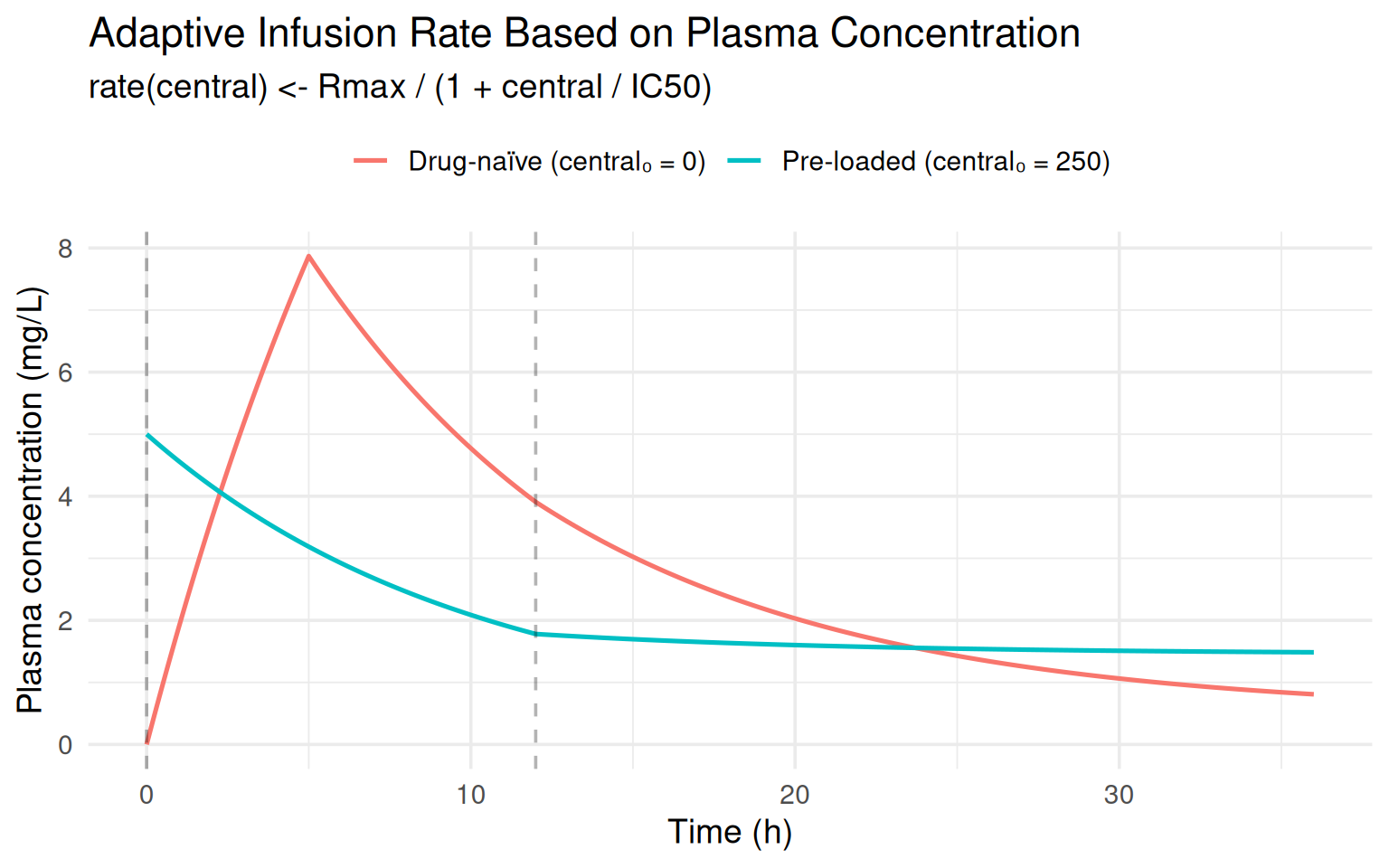
The pre-loaded subject receives a much slower infusion (the
denominator $1 + C/$ is large), producing a markedly
different PK profile from the same dosing regimen — all handled
automatically by rxode2 evaluating the rate expression at dose time.
Conclusion
rxode2 5.0.2 adds a powerful feature to rxode2: the ability to make
dosing properties — infusion rate, infusion duration, bioavailability,
absorption lag time, and model event times — depend on the current
state of the ODE system.
This required changes deep in the event-sorting and dose-firing
machinery, including runtime re-sorting of infusion stop events and
careful evaluation of state vectors at the correct time points.
The result is a clean, intuitive syntax (rate(cmt) <- expr,
dur(cmt) <- expr, f(cmt) <- expr, alag(cmt) <- expr) that
works exactly the same whether the expression involves only parameters
or also state variables.
To try it out, install the latest version of rxode2 from
CRAN.
As always, please report any issues on GitHub.
Session Information
sessionInfo()
#> R version 4.5.3 (2026-03-11)
#> Platform: x86_64-pc-linux-gnu
#> Running under: Ubuntu 24.04.4 LTS
#>
#> Matrix products: default
#> BLAS:   /usr/lib/x86_64-linux-gnu/blas/libblas.so.3.12.0
#> LAPACK: /usr/lib/x86_64-linux-gnu/lapack/liblapack.so.3.12.0  LAPACK version 3.12.0
#>
#> locale:
#>  [1] LC_CTYPE=en_US.UTF-8       LC_NUMERIC=C
#>  [3] LC_TIME=en_US.UTF-8        LC_COLLATE=en_US.UTF-8
#>  [5] LC_MONETARY=en_US.UTF-8    LC_MESSAGES=en_US.UTF-8
#>  [7] LC_PAPER=en_US.UTF-8       LC_NAME=C
#>  [9] LC_ADDRESS=C               LC_TELEPHONE=C
#> [11] LC_MEASUREMENT=en_US.UTF-8 LC_IDENTIFICATION=C
#>
#> time zone: America/Chicago
#> tzcode source: system (glibc)
#>
#> attached base packages:
#> [1] stats     graphics  grDevices utils     datasets  methods   base
#>
#> other attached packages:
#> [1] tidyr_1.3.2   dplyr_1.2.0   ggplot2_4.0.2 rxode2_5.0.2
#>
#> loaded via a namespace (and not attached):
#>  [1] sass_0.4.10           generics_0.1.4        blogdown_1.23
#>  [4] lattice_0.22-9        digest_0.6.39         magrittr_2.0.4
#>  [7] evaluate_1.0.5        grid_4.5.3            RColorBrewer_1.1-3
#> [10] bookdown_0.46         fastmap_1.2.0         lotri_1.0.3
#> [13] qs2_0.1.7             jsonlite_2.0.0        rxode2ll_2.0.14
#> [16] backports_1.5.0       purrr_1.2.1           scales_1.4.0
#> [19] jquerylib_0.1.4       cli_3.6.5             crayon_1.5.3
#> [22] rlang_1.1.7           units_1.0-0           withr_3.0.2
#> [25] cachem_1.1.0          yaml_2.3.12           otel_0.2.0
#> [28] tools_4.5.3           memoise_2.0.1         checkmate_2.3.4
#> [31] vctrs_0.7.2           R6_2.6.1              lifecycle_1.0.5
#> [34] stringfish_0.18.0     PreciseSums_0.7       pkgconfig_2.0.3
#> [37] RcppParallel_5.1.11-2 pillar_1.11.1         bslib_0.10.0
#> [40] gtable_0.3.6          data.table_1.18.2.1   glue_1.8.0
#> [43] Rcpp_1.1.1            xfun_0.57             tibble_3.3.1
#> [46] tidyselect_1.2.1      sys_3.4.3             knitr_1.51
#> [49] farver_2.1.2          dparser_1.3.1-13      htmltools_0.5.9
#> [52] nlme_3.1-168          labeling_0.4.3        rmarkdown_2.30
#> [55] compiler_4.5.3        S7_0.2.1